What are Six Sigma Statistics: Complete Guide

Estimated reading time: 8 minutes

A Guide to Six Sigma Statistics

Statistics are the foundation of Lean Six Sigma projects. This allows us to express the data that makes up X and Y using numbers. A Six Sigma Statistic is an integral part of every organization’s day-to-day operations. Six Sigma projects are based on numbers, diagrams, and data. Six Sigma professionals and all stakeholders need to be familiar with basic Lean Six Sigma statistical analysis.

Types of Data in Six Sigma

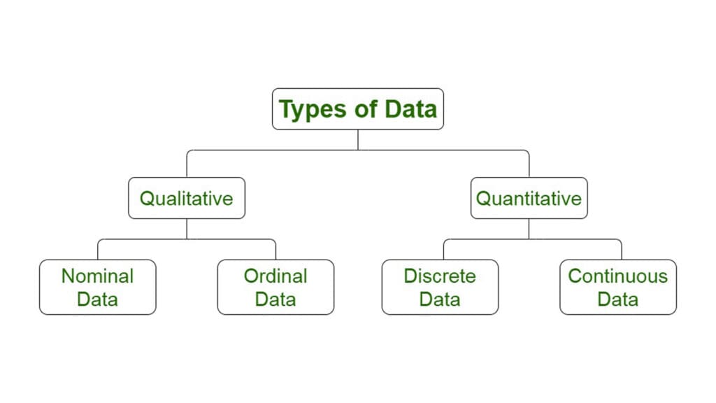
Data can be either quantitative or qualitative. It could be a number or a measurement.

Qualitative: This data is also called non-numeric and describes the characteristics of a value. Each data point can be placed in one of several possible categories.

• Nominal Data: This type of descriptive data can be used to refer to the names and labels of data points. For example, hair color could be black or brown, and gender could be male or female.
• Ordinal Data: Oral data gives good information about the order in which choices are made. It arranges information in a certain order but does not indicate a relationship between items. Ex: Pass or fail, customer service good or bad, etc.

Quantitative Data: Also known as numerical data. Data points can be either measured or counted. It is not like Qualitative data because it can contain infinite numbers of possible categories in which each data point could be placed. Quantitative data can be further subdivided into two types of data:

• Distinct data: Data is considered discrete when the numbers or counts are whole numbers. You could use this data to determine customer complaints and weekly defects.
• Continuous data: The data is continuous when the measurement takes on any value. Usually, this range is within a certain range. For example, Stack height, distance, cycle time, etc.

Basic Types of Lean Six Sigma Statistics

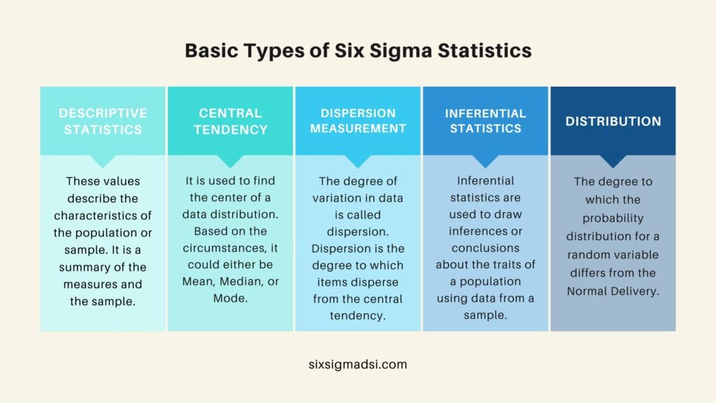
Lean Six Sigma is a methodology that combines Lean principles and Six Sigma tools to improve process efficiency and reduce defects. In the context of Lean Six Sigma, various statistical tools (diagrams) are used to analyze and measure process performance. Here are some basic types of statistics commonly employed in Lean Six Sigma:

Descriptive statistics

Descriptive statistics are used to summarize and describe the main features of a data set. Common measures include mean, median, mode, range, standard deviation, and variance.

Central Tendency

The statistical measure is used to find the center of data distribution in Six Sigma statistical analysis. Based on the circumstances, the measure central tendency could either be Mean, Median, or Mode.

• Mean: The sum of all data values divided by the number of data points is called the mean.
• Median: The median value is the average value of the data when it is ordered from least to most or vice versa. If there are even data values, the median will be the average of those two values.
• Mode: This is the value that most often appears in the data set.

Dispersion measurement

• Dispersion measures quantify the spread or variability of data points in a dataset, providing insights into the distribution of values.
• Examples:
  • Range: The difference between the maximum and minimum values.
  • Variance: A measure of the average squared difference from the mean.
  • Standard Deviation: The square root of the variance.

Inferential statistics

• Inferential statistics involve making inferences and predictions about a population based on a sample of data. These statistics help draw conclusions beyond the observed data.
• Examples:
  • Hypothesis Testing: Making decisions about a population based on sample data.
  • Confidence Intervals: Estimating a range in which a population parameter is likely to fall.
  • Regression Analysis: Predicting the relationship between variables.

Shape of Distribution

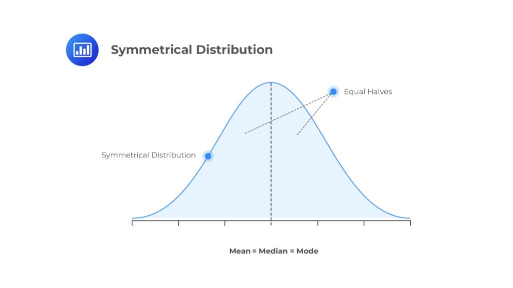
In the context of Six Sigma, the shape of the distribution is often associated with the normal distribution, also known as the Gaussian distribution. The normal distribution has a specific bell-shaped curve, and it is frequently used in Six Sigma diagrams for several reasons:

1. Symmetry: The normal distribution is symmetric, meaning that the left and right sides of the distribution are mirror images of each other. This symmetry simplifies statistical analysis and makes it easier to interpret results in Six Sigma diagrams.
2. Central Tendency Measures: In a normal distribution, the mean, median, and mode are all located at the center of the distribution. This central tendency allows for a clear understanding of the average or typical value.
3. Control Limits in Statistical Process Control (SPC): Many statistical process control charts, a key tool in the Control phase of Six Sigma (DMAIC), assume a normal distribution. Control limits on these charts are often based on the properties of the normal distribution.
4. Process Capability Indices: Indices like Cp, Cpk, Pp, and Ppk, which are used to assess and quantify process capability, are based on the assumption of a normal distribution. These indices compare the spread of the process to the specifications.

The data in a bite

Six Sigma statistical analysis is a great way, to sum up, the data in Six Sigma Statistic projects. The graphical analysis takes the data and creates images that help to understand the relationships between the process parameters. Graphical analysis is often the first step in any problem-solving process.

Box and Whisker plot is also known as Box and Whisker plot. It is a pictorial representation of continuous data. The box plot displays the Max, Min, and median values, as well as the interquartile range Q1, Q3, and outlier.

A time series plot is a line graph that plots data over time. It allows you to see the patterns in the time series. They don’t have control limits so we can’t judge if the process is stable.

A histogram shows a graphic representation of a frequency distribution. It’s rectangular with the class intervals being the bases and the frequencies as the heights. There is no space between the two rectangles that follow it.

Pareto Chart also known as the 80-20 Rule. It is a combination bar chart and a line chart. The actual data are in descending order with a bar chart and the cumulative data are in ascending order with a line graph.

Six Sigma Statistic Data Symbols

In Six Sigma, various statistical data symbols are used to represent different parameters, measurements, and characteristics of a process. These symbols are commonly employed in statistical analyses, process documentation, diagrams, and communication among Six Sigma practitioners.

( \mu ):

• Symbol: Mu (Greek letter)
• Representation: Represents the population mean. In statistical terms, it is the average of all data points in a population.

( \bar{x} ):

• Symbol: x-bar (pronounced “x-bar”)
• Representation: Represents the sample mean. It is the average of a sample of data points from a population.

( \sigma ):

• Symbol: Sigma (Greek letter)
• Representation: Represents the population standard deviation. It quantifies the amount of variation or dispersion in a population.

( s ):

• Symbol: Lowercase “s”
• Representation: Represents the sample standard deviation. It is an estimate of the population standard deviation based on a sample.

( Z ):

• Symbol: Z (standard score)
• Representation: Represents the number of standard deviations a data point is from the mean in a standard normal distribution. It is used in statistical process control and hypothesis testing.

( N ):

• Symbol: N
• Representation: Represents the sample size. It is the number of observations in a sample.

( Cp ) and ( Cpk ):

• Symbol: Cp and Cpk
• Representation: Represents process capability indices. Cp measures the potential capability of a process, while Cpk accounts for process centering.

( P ), ( Pp ), and ( Ppk ):

• Symbol: P, Pp, and Ppk
• Representation: Represents process capability indices for discrete data, particularly in the context of defect rates.

( DPMO ):

• Symbol: DPMO (Defects Per Million Opportunities)
• Representation: Represents the number of defects per million opportunities. It is used to assess process performance.

( AQL ) and ( LSL/USL ):

• Symbol: AQL (Acceptable Quality Level), LSL (Lower Specification Limit), USL (Upper Specification Limit)
• Representation: AQL represents the maximum acceptable defect rate. LSL and USL represent the lower and upper limits specified by the customer.

Related Articles

• ‘Median’ as a Measure of Central Tendency
• Central Tendency
• Using Standard Deviation as a Measure of Dispersion
• Using Range as a Measure of Dispersion
• Range