
Discrete data is information you count, not measure. It exists only in whole, separate values, like the number of defective parts on a shift or the number of customer complaints in a week. You cannot have 3.5 defects or half a complaint.
Discrete data matters in Six Sigma because it determines which control chart, which capability formula, and which hypothesis test a team is allowed to use. Get the data type wrong and every downstream calculation, from a P-Chart to a sigma level, becomes invalid. This guide covers the types of discrete data, real business examples, how to chart and validate it, and the mistakes that quietly derail Six Sigma projects.
| Aspect | Discrete Data | Continuous Data |
| Definition | Countable, whole-number values | Measurable values on a continuous scale |
| Example | Number of defects, number of employees hired | Cycle time, temperature, weight |
| Values between points | None (no 4.5 defects) | Infinite (4.5 seconds is valid) |
| Common charts | P, NP, C, U charts, bar charts, Pareto charts | I-MR, X-bar R, X-bar S charts, histograms |
| Statistical distribution | Binomial or Poisson | Normal (or transformed to approximate normal) |
| Sample size needed for reliable analysis | Larger (often 100+ units) | Smaller (often 30-50 units) |
| Six Sigma capability metric | DPMO, sigma level (Z), Rolled Throughput Yield | Cp, Cpk, Pp, Ppk |
Table of contents
Key Takeaways
- Discrete data is countable and made up of whole numbers with no possible values in between, such as 2 defects or 3 defects, never 2.5.
- Discrete data is also called attribute data in Six Sigma and quality management contexts.
- The four attribute control charts, P, NP, C, and U, exist specifically to monitor discrete data over time.
- Discrete data requires larger sample sizes than continuous data to detect the same size of process shift, which is why experienced Black Belts try to convert attribute measurements into continuous ones whenever possible.
- Before trusting discrete data at all, Six Sigma teams validate the people or systems collecting it using an Attribute Agreement Analysis (Kappa study).
What Is Discrete Data?
Discrete data is a type of quantitative data made up of countable, whole-number values with no possible value between them. If you count 7 late shipments in a week, the next possible count is 6 or 8, never 6.5. This is what separates discrete data from continuous data, which can take any value within a range, including decimals and fractions.
Discrete data is a synonym for attribute data in most Six Sigma and Lean manufacturing contexts, though a small distinction exists. Attribute data specifically refers to pass/fail or good/bad classifications, while discrete data more broadly covers any countable whole number, including counts that are not binary classifications, such as the number of calls received by a support center in an hour.
Six Sigma Development Solutions Inc. teaches this distinction on day one of Green Belt training, because a team that mislabels its data type will select the wrong control chart and the wrong capability formula for the rest of the project. That single classification error can invalidate months of process data.

Public, Onsite, Virtual, and Online Six Sigma Certification Training!
- We are accredited by the IASSC.
- Live Public Training at 52 Sites.
- Live Virtual Training.
- Onsite Training (at your organization).
- Interactive Online (self-paced) training,
Discrete Data vs. Continuous Data: What Actually Changes
The difference between discrete and continuous data is not academic. It changes four practical things on a Six Sigma project: the chart you build, the sample size you need, the statistical distribution behind your math, and the test you run to compare two processes.
- Values: Discrete data is counted (2 defects, 5 employees). Continuous data is measured (2.3 seconds, 5.7 kilograms).
- Data type: Discrete values are integers. Continuous values usually carry decimals.
- Underlying distribution: Discrete data typically follows a binomial distribution (pass/fail counts) or a Poisson distribution (rare event counts, like defects per unit). Continuous data typically follows a normal distribution, or is transformed to approximate one.
- Sample size: According to the American Society for Quality, attribute (discrete) sampling plans generally require substantially larger sample sizes than variable (continuous) sampling plans to detect the same magnitude of process change, because a count carries less information per data point than a direct measurement.
| Factor | Discrete (Attribute) Data | Continuous (Variable) Data |
| How it’s collected | Counting, checking, classifying | Measuring with an instrument |
| Typical distribution | Binomial or Poisson | Normal |
| Information per data point | Lower | Higher |
| Sample size to detect a shift | Larger | Smaller |
| Six Sigma control charts | P, NP, C, U | I-MR, X-bar R, X-bar S |
Also Read: Data Distributions in Six Sigma: Types, How to Identify Them, and Why They Matter
Types of Discrete Data
Not all discrete data behaves the same way statistically, and Six Sigma teams need to know which sub-type they are working with before picking a chart.
Binary (Pass/Fail) Discrete Data
Each unit gets one of two classifications. A part is defective or it is not. A call resolves on first contact or it does not. Binary discrete data follows a binomial distribution and feeds directly into P-Charts and NP-Charts.
Count Discrete Data
This tracks how many times something happens, without a natural upper limit, like the number of scratches on a car door or billing errors on an invoice. Count data typically follows a Poisson distribution and feeds C-Charts and U-Charts.
Categorical (Nominal) Discrete Data
This groups observations into named categories with no numeric order, such as defect type (scratch, dent, misalignment) or department (sales, billing, support). A Pareto chart is the standard tool for prioritizing the most frequent category.
Ordinal Discrete Data
This ranks categories in a meaningful order, such as a customer satisfaction rating of 1 through 5. The values stay discrete, but their order carries information that nominal data does not.
Real Business Examples of Discrete Data
Tickets Sold Per Event
A venue tracking tickets sold for a show is recording discrete data. It is discrete because the value cannot land between two whole numbers; a venue sells 412 tickets or 413, never 412.5.
Number of Employees
Headcount is a classic example of discrete data. Companies track it to manage span-of-control ratios, staffing budgets, and hiring pace against growth targets.
Product Reviews Received
The number of reviews a product receives in a given week is discrete data. Customer experience teams use this count, often alongside the discrete rating each reviewer selects, to track engagement trends over time.
Employee Hire Dates and Tenure Counts
The number of days, weeks, or months an employee has been with a company is discrete data used to trigger onboarding milestones and benefits eligibility.
Manufacturing Defects Per Batch
A production line recording defective units in each batch of 500 generates discrete data that feeds directly into a P-Chart or NP-Chart, depending on whether batch size stays constant.
Customer Complaints Per Month
A call center tracking complaints logged each month works with discrete count data, typically visualized on a C-Chart when the reporting period (a month) stays a fixed size.
Also Read: Data Collection Plan in Six Sigma: What It Is, Template, and How to Build One
How to Visualize Discrete Data
Discrete data is almost always visualized differently than continuous data, because the goal is to compare distinct categories or counts rather than show a smooth distribution.
- Bar graphs: Compare discrete categories side by side, such as defects by shift or sales by product line. Each bar represents one distinct value, with gaps between bars to reflect the non-continuous nature of the data.
- Pareto charts: A specialized bar chart, ranked from most frequent to least frequent, used to identify the “vital few” defect categories responsible for most of the problem. This is a core Six Sigma Measure-phase tool for categorical discrete data.
- Frequency tables: A simple two-column table pairing each category with its count, useful for both categorical and count discrete data before it goes into a chart.
- Run charts: Plot discrete counts over time in sequence, useful as a first look before formal control limits are calculated.
Discrete Data in Six Sigma: Choosing the Right Control Chart

This is where most online explanations of discrete data stop short, and where Six Sigma projects most often go wrong. Picking the correct attribute control chart depends on two questions: are you counting defective units or individual defects, and does your sample size stay constant?
| Chart | Counts | Sample Size | Distribution | Example Use Case |
| P-Chart | Proportion of defective units | Varies | Binomial | Percentage of loan applications rejected per week, when weekly volume changes |
| NP-Chart | Number of defective units | Constant | Binomial | Number of defective circuit boards out of a fixed batch of 200 |
| C-Chart | Number of defects (a unit can have more than one) | Constant unit size | Poisson | Number of scratches found on inspected car doors, one door per inspection |
| U-Chart | Defects per unit | Varies | Poisson | Software bugs per 1,000 lines of code, when code volume varies by release |
A practical rule Six Sigma Black Belts use: if you are asking “is this item good or bad,” reach for a P-Chart or NP-Chart. If you are asking “how many things are wrong with this item,” reach for a C-Chart or U-Chart. Getting this wrong produces control limits that are too tight or too loose, which means the chart signals false alarms or, worse, misses a real process shift entirely.
Measuring Process Capability with Discrete Data
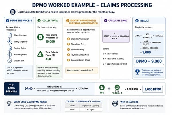
Once a discrete data process is stable on a control chart, Six Sigma teams still need to know how capable it is against customer requirements. Because discrete data has no upper and lower specification limits the way continuous data does, capability is measured differently.
- DPMO (Defects Per Million Opportunities): Counts actual defects against the total number of opportunities for a defect to occur, then scales the result to a per-million basis so processes of different sizes can be compared on the same footing.
- Sigma Level (Z): Converts DPMO into a standard sigma benchmark. A process producing 66,807 DPMO sits at roughly 3 sigma, while a process producing 3.4 DPMO sits at 6 sigma, using the standard 1.5 sigma long-term shift convention.
- Rolled Throughput Yield (RTY): The probability that a unit passes through every step of a process with zero defects, calculated by multiplying the first-pass yield of each individual step.
Worked example: A claims processing team reviews 1,000 claims. Each claim has 4 fields that could be entered incorrectly (4 opportunities per unit), giving 4,000 total opportunities. The team finds 48 errors. DPMO = (48 / 4,000) x 1,000,000 = 12,000 DPMO, which corresponds to a sigma level of approximately 3.75. That single number tells leadership exactly where the process ranks and how much room for improvement remains.
Validating Discrete Data Before You Trust It: Attribute Agreement Analysis
Continuous data comes from a calibrated instrument. Discrete data usually comes from a human judgment call, an inspector deciding “pass” or “fail,” a support agent classifying a ticket as “resolved” or “escalated.” That judgment can be inconsistent, which is why Six Sigma practitioners run an Attribute Agreement Analysis, also called a Kappa study, before trusting discrete data at all.
The Kappa statistic measures how much two inspectors agree with each other, and how much a single inspector agrees with their own earlier decision, after removing the agreement that would happen by pure chance. Kappa values range from -1 to +1, and a value above 0.75 is generally considered strong agreement for a production measurement system. If Kappa comes back low, the discrete data feeding your control chart and your DPMO calculation is unreliable, no matter how clean the counts look on paper.
Common Mistakes Teams Make With Discrete Data
- Treating a rating scale as continuous data. A 1-to-5 satisfaction score is discrete and ordinal, not continuous, and running a t-test on it without justification produces misleading conclusions.
- Using a P-Chart when sample size is fixed. An NP-Chart is simpler and more appropriate when every subgroup has the same size.
- Skipping the Attribute Agreement Analysis. Teams that never validate inspector consistency often “fix” a process that was never broken, only inconsistently judged.
- Under-sampling. Because discrete data carries less information per observation than continuous data, small sample sizes produce wide, unreliable control limits.
- Converting discrete data to continuous data incorrectly. Averaging a pass/fail score into a percentage does not make the underlying data continuous; the statistical rules for discrete data still apply.
Frequently Asked Questions on Discrete Data
Is discrete data the same as attribute data?
In practice, yes. Six Sigma and quality management use “discrete data” and “attribute data” interchangeably, though attribute data more narrowly refers to pass/fail or good/bad classifications while discrete data covers any countable whole number.
Can discrete data have decimals?
No. Discrete data only takes whole-number values because it comes from counting. An average calculated across many discrete values, such as 2.3 defects per batch, can be a decimal, but each individual observation cannot.
Which control chart should I use for discrete data?
Use a P-Chart for defective units with a varying sample size, an NP-Chart for defective units with a constant sample size, a C-Chart for counting defects on a constant unit size, and a U-Chart for defects per unit with a varying sample size.
Why does discrete data need larger sample sizes than continuous data?
A single continuous measurement carries more statistical information than a single pass/fail count, so detecting the same size of process shift with discrete data requires more observations to reach the same confidence level.
What is the difference between DPMO and sigma level?
DPMO is the raw count of defects scaled to one million opportunities. Sigma level converts that DPMO figure into a standardized benchmark (from 1 sigma to 6 sigma) so processes of different sizes and industries can be compared directly.
Final Words
Discrete data looks simple on the surface, a count of tickets, employees, or defects, but it drives some of the most consequential decisions on a Six Sigma project: which control chart to build, how much data to collect, and whether a process is truly capable. Teams that classify their data correctly from the start avoid months of rework on charts and capability studies that never should have been built that way.
Six Sigma Development Solutions Inc. has taught data classification, control charts, and capability analysis to practitioners across onsite, live virtual, public, and online formats for over two decades. Our Green Belt and Black Belt certification courses walk you through real discrete and continuous datasets, not just theory, so you leave able to build the correct chart the first time. View our upcoming Green Belt and Black Belt training schedule and get $500 off your next class.
About Six Sigma Development Solutions, Inc.
Six Sigma Development Solutions, Inc. offers onsite, public, and virtual Lean Six Sigma certification training. We are an Accredited Training Organization by the IASSC (International Association of Six Sigma Certification). We offer Lean Six Sigma Green Belt, Black Belt, and Yellow Belt, as well as LEAN certifications.
Book a Call and Let us know how we can help meet your training needs.


