Table of contents
Using “Standard Deviation” as a Measure of Data Spread or Dispersion
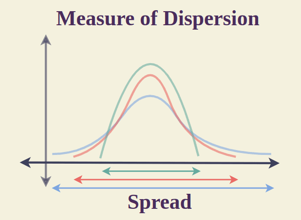
A measure of dispersion in a standard deviation units chart tells you the sign spread of the data. It is important to know the standard deviation rule spread of your data when describing your data set. Most describe a set of data by using only the mean or median leaving out a description of the spread.
There are two main measures of spread or dispersion:
In this article, we will discuss the Standard Deviation of the Distribution
The standard deviation(s) is the most common measure of dispersion. Standard deviation tells you how spread out or dispersed the data is in the data set. It is a measure of how far each observed value in the data set is from the mean. In any distribution, theoretically, 99.73% of values will be within +-3 standard deviations of the mean.

What is Standard Deviation (SD)?
The standard deviation is a statistical measure of dispersion in a dataset compared to the mean. It is calculated by taking the square root variance. The standard deviation is determined by taking the square root variance.
The standard deviation will be higher if the data points are farther from the mean.
What is Standard Deviation?
The standard deviation sign is a financial statistic that when applied to an investment’s annual rate of return, sheds some light on its historic volatility.
The Standard deviation rule is a measure of the difference between the price of each security and the average price. This shows the price range. A volatile stock, for example, has a large standard deviation. However, the deviation of stable blue chip stocks is typically low.
What is Dispersion?
In statistics, dispersion describes how data are spread across different categories. The size of the distribution values expected for the data set is calculated. Dispersion is defined as “numerical data that are likely to vary in any instance where average value assumptions “.
Statistics’ dispersion of data helps you to understand a dataset more easily by classifying it into its own specific criteria such as variance, standard deviation, and range.
The dispersion measures are a collection of metrics that help determine the quality and quantity of data. Dispersion is a concept that cannot be skipped in most data science courses.
Measures for Dispersion
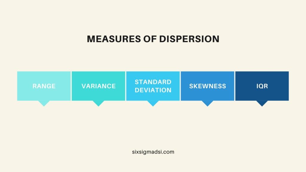
Measures of dispersion are almost always the same size as the quantity that is being measured. Many Measures of dispersion have been found to help us gain more insight into our data.
- Range
- Variance
- Standard Deviation
- Skewness
- IQR

Measures of Dispersion Types
Measures of dispersion are divided into two categories that offer different ways to measure the diversity of data. This is mostly used in biological statistics. You can classify them easily by determining whether or not they contain units.
As per the above, the data can be divided into two categories:
- Absolute measures of dispersion
- Relative measures of dispersion
Absolute measures of dispersion
Absolute measures of dispersion are expressed in the same units as the original dataset. The Absolute Measurement of Dispersion can be expressed as the average of dispersion quantities such as Standard deviation or Mean Deviation. The Absolute Dispersion Measure can be expressed using units like rupees, centimeters, marks, kilograms, and other quantities depending on the situation.
Relative measures of dispersion
The values of Relative Measures of Dispersion are not units. Comparing the distribution of multiple datasets is done using a relative measure of dispersion.
The only difference between the absolute measure of dispersion and the relative measure of dispersion is in the quantity of measurement.
Types of relative measure of dispersion: The coefficient is calculated by comparing two series that have a large difference in average.
When comparing 2 series of measurements with different units of measurement, the coefficients of dispersion are most useful.
Why is the Standard Deviation Rule Important in Lean Six Sigma?
Let’s look at an example. Let’s say I owned a company that produced widgets as a sub-component for other parts. Every time a widget is produced, a system records the time it took from start to finish of the widget. The requirements for the time to complete a widget are no less than 6 minutes and no more than 18 minutes.
In the below example, we calculate the standard deviation as 1.5 minutes from a sample of 60 widgets.
You can see from this process that it can perform within the specification limits or the process tolerance.
What happens if the standard deviation units increase?
As the standard deviation chart of the process increases (which means that variation in the process is increasing), the width of the process grows, bringing it closer to exceeding the process tolerance.
These illustrations show that knowing the standard deviation and tolerance of a process can show the performance of the process. Knowing the performance of a process is critical in a Lean Six Sigma project.


