
A histogram is a type of bar chart that represents the distribution of numerical data by displaying the frequency of data within specified ranges, known as bins. It provides a visual interpretation of numerical data by indicating the number of data points that lie within a range of values.
A histogram visually shows data distribution. It uses bars to represent frequency. The height of each bar shows how often values occur. The x-axis shows value ranges, called bins. The y-axis shows the frequency or count. Histograms help us see patterns in data.
Table of contents
- Introducing Skewness
- Understanding Right-Skewed Histograms
- Difference Between Right-Skewed and Left-Skewed Histogram
- How to Identify Right-Skewed Data?
- Handling Right-Skewed Data
- Real-World Examples
- How to Create a Right-Skewed Histogram
- Statistical Implications of Right-Skewed Data
- Facts on Right-Skewed Histogram
- Final Words
- Related Articles
Introducing Skewness
Skewness describes the symmetry of a data set. A symmetrical distribution looks like a bell curve. Both sides are mirror images. A skewed distribution is not symmetrical. It has a “tail” that extends more on one side.
Understanding Right-Skewed Histograms
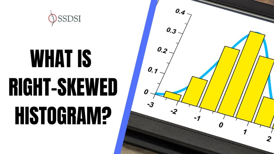
A right-skewed histogram, is also referred to as a positively skewed histogram. A right-skewed histogram has a longer tail on the right side. Most data points cluster on the left. This means many lower values exist. Fewer higher values extend the tail to the right. It is also known as a positively skewed histogram.
Visualizing Right Skewness
Imagine a hill with a long, gentle slope on the right. The peak of the hill is on the left. The slope extends to the right. This is a right-skewed shape.
Right Skewed Histogram Diagram
- The diagram will have a horizontal x-axis and a vertical y-axis.
- The x-axis will show the value of the data.
- The y-axis will show the frequency.
- The bars of the histogram will have the tallest bars on the left side of the graph, and the height of the bars will decrease as you move to the right side of the graph.
- The tail of the graph will extend further to the right.
Key Characteristics of Right-Skewed Histograms
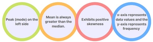
- Shape and Appearance: The histogram has a peak (mode) on the left side. The tail extends out to the right, indicating that there are a few large values that are different from the majority of the data points. As you move from left to right, the frequency of data points decreases.
- Mean, Median, and Mode: In a right-skewed distribution, the mean is always greater than the median. The median will be greater than the mode. This occurs because the mean is affected by the outliers (the larger values) in the right tail.
- Skewness: A right-skewed histogram exhibits positive skewness. This means that the tail on the right side of the distribution is longer than the tail on the left. The skewness coefficient for a right-skewed distribution will be positive, indicating that the data are skewed towards larger values.
- Visual Indicators: On a histogram, the x-axis represents data values divided into bins, while the y-axis represents frequency or count. For a right-skewed histogram, the bars on the left side are taller (indicating higher frequencies of smaller values), while the bars on the right side are shorter but extend farther.
Difference Between Right-Skewed and Left-Skewed Histogram
| Feature | Right-Skewed Histogram | Left-Skewed Histogram |
| Tail Direction | The tail extends to the left (towards lower values). | The peak is located on the left side of the graph. |
| Data Concentration | Most data points are concentrated on the left side of the distribution. | Most data points are concentrated on the right side of the distribution. |
| Mean, Median, Mode Relationship | Mean > Median > Mode | Mode > Median > Mean |
| Common Name | Positively skewed | Negatively skewed |
| Visual Peak Location | The peak is located on the right side of the graph. | income distributions, durations of website visits, and some test scores. |
| Affect of Outliers | High-value outliers pull the mean towards the higher values, increasing the mean. | Low-value outliers pull the mean towards the lower values, decreasing the mean. |
| Effect on Statistical Analysis | May require data transformation (e.g., logarithmic) for certain statistical tests that assume normality. | May require data transformation for certain statistical tests that assume normality. |
| A long right tail means less frequency of high values | long left tail means less frequency of low values | Typical real-world examples |
| Interpretation of the tails | Long right tail means less frequency of high values | A long right tail means less frequency of high values |
| Influence on the Median | The median is influenced, but less so than the mean, and shifts towards the right tail. | The median is influenced, but less so than the mean, and shifts towards the left tail. |
| Skewness Value | Positive skewness value | The tail extends to the right (towards higher values). |
How to Identify Right-Skewed Data?
There are several ways to determine if a dataset follows a right-skewed distribution:
- Histogram Inspection: The easiest way to identify right-skewness is by plotting a histogram. If the tail of the histogram is longer on the right side than on the left, the data is right-skewed.
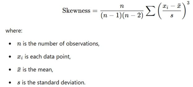
- Skewness Coefficient: The skewness coefficient is a statistical measure that quantifies the asymmetry of a distribution. If the skewness coefficient is positive, the distribution is right-skewed. The formula for skewness is:
- Measures of Central Tendency: In a right-skewed dataset, the mean will be greater than the median. This difference indicates that the larger values in the right tail are pulling the mean towards the higher end.
- Boxplot Analysis: A boxplot can also help identify skewness. In a right-skewed dataset, the boxplot will show the median closer to the lower end of the box, with a longer whisker on the right side.
Handling Right-Skewed Data
When dealing with right-skewed data, there are several strategies you can employ to manage the skewness and make the data more suitable for analysis:
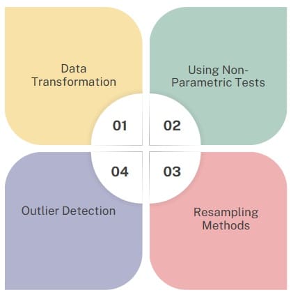
- Data Transformation:
- Logarithmic Transformation: One common method to handle right-skewed data is applying a logarithmic transformation. Taking the logarithm of each data point reduces the influence of large values and compresses the tail, making the data more symmetric.
- Square Root Transformation: This method is also useful for right-skewed data. It’s often used for count data (e.g., the number of occurrences of an event).
- Box-Cox Transformation: This is a more generalized transformation that can handle a variety of skewed distributions. It is particularly useful when the dataset contains both positive and negative values.
- Using Non-Parametric Tests:
When skewness is severe, using non-parametric tests instead of traditional parametric tests ensures more reliable results. Non-parametric methods do not assume normality and are more robust to skewness. - Resampling Methods:
Techniques such as bootstrapping or permutation tests can be used to estimate confidence intervals or p-values without making assumptions about the underlying distribution of the data. - Outlier Detection:
In some cases, the right tail may be caused by extreme outliers. Identifying and removing outliers can reduce the skewness in the data. However, care should be taken to ensure that the outliers are truly erroneous and not part of the natural variation in the data.
Real-World Examples
- Income Distribution: Most people earn average incomes. A few earn very high incomes. This creates a right-skewed distribution.
- Test Scores: Many students score average. Few students score very high. This is another right-skewed pattern.
- Website Traffic: Many days have low traffic. A few days have very high traffic. This forms a right-skewed graph.
- Retirement Ages: Many people retire around a certain age. Some people retire much later. This creates a right skewed distribution.
How to Create a Right-Skewed Histogram
A right-skewed histogram displays data where the majority of values are concentrated on the left side of the graph, with a tail extending towards higher values on the right. This visual representation reveals that while many data points fall within the lower range, a smaller number of data points have significantly higher values. To create such a histogram, you begin by gathering your numerical data.
Next, you divide the range of your data into equal intervals, called bins, and count how many data points fall into each bin. These counts represent the frequency of data within each interval. You then draw a graph with a horizontal x-axis, representing the data values or bins, and a vertical y-axis, representing the frequency.
For each bin, a bar is drawn with a height corresponding to its frequency. Upon completion, the histogram will reveal a peak on the left side and a tail extending to the right, signifying right skewness. This pattern indicates that the mean of the data is typically greater than the median, as the high values in the right tail pull the average towards them.
Also Read: Lean Six Sigma Certification Programs, Irvine, California
Statistical Implications of Right-Skewed Data
Understanding the implications of right-skewed data is important for statistical analysis. Skewness affects the choice of statistical methods, and misinterpreting the distribution can lead to incorrect conclusions.
- Mean vs. Median: In right-skewed data, the mean is typically greater than the median. This happens because the mean is sensitive to extreme values (outliers) in the tail. The median, on the other hand, is more robust and reflects the central tendency better in skewed distributions.
- Impact on Statistical Tests: Many parametric tests (e.g., t-tests, ANOVA) assume normality in the data. When the data is right-skewed, these tests may not be appropriate, as they may lead to inaccurate results. For skewed data, non-parametric tests such as the Mann-Whitney U test or the Kruskal-Wallis test are often used. These tests do not rely on the assumption of normality and are more appropriate for skewed distributions.
- Regression Analysis: In regression analysis, the presence of skewness can impact the residuals (the difference between the observed and predicted values). Skewed residuals violate the assumption of normality, which is essential for accurate hypothesis testing and confidence intervals. To address this, one might apply transformations to normalize the data or use robust regression techniques that can handle skewed data.
Facts on Right-Skewed Histogram
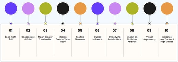
Long Right Tail: The defining characteristic is a tail that extends significantly towards higher values on the right side of the graph.
Concentrated Data: Most data points are clustered on the left side, indicating a higher frequency of lower values.
Mean Greater Than Median: The mean (average) is pulled to the right by high values, resulting in the mean being larger than the median (middle value).
Median Greater Than Mode: The median typically exceeds the mode (most frequent value), which is located at the peak of the histogram.
Positive Skewness: Right-skewed distributions are also known as positively skewed distributions.
Outlier Influence: High-value outliers significantly affect the mean, contributing to the long right tail.
Underlying Distributions: Right skewness often arises from data that follows distributions like the exponential, log-normal, or Weibull distributions.
Impact on Statistical Analysis: Right skewness can affect the validity of statistical tests that assume a normal distribution, often necessitating data transformations.
Visual Asymmetry: The histogram exhibits a clear lack of symmetry, with a distinct peak on the left and a gradual decline towards the right.
Indicates Less Frequent High Values: The right tail signifies that while high values exist, they occur less frequently than lower values.
Final Words
Right-skewed histograms are a fundamental concept in statistics. They occur when the distribution of data has a long tail on the right side, indicating that there are a few extreme values that are much larger than most of the data points.
Recognizing right-skewed distributions is essential for accurate data analysis, as it influences the choice of statistical tests and the interpretation of central tendency measures.

About Six Sigma Development Solutions, Inc.
Six Sigma Development Solutions, Inc. offers onsite, public, and virtual Lean Six Sigma certification training. We are an Accredited Training Organization by the IASSC (International Association of Six Sigma Certification). We offer Lean Six Sigma Green Belt, Black Belt, and Yellow Belt, as well as LEAN certifications.
Book a Call and Let us know how we can help meet your training needs.