
The Box-Cox transformation is a statistical method that converts non-normal data into a shape that closely resembles a normal distribution. Statisticians George Box and David Cox introduced it in a 1964 paper. Many statistical tools, including hypothesis tests and process capability studies, assume normally distributed data. When a data set fails that assumption, a Box-Cox transformation can often fix it, opening the door to tests and control charts that would otherwise give misleading results.
Table of contents
What is a Box-Cox transformation?
The Box-Cox transformation is a mathematical method that raises data to a power, denoted by lambda, to make a skewed or non-normal data set resemble a normal distribution. George Box and David Cox published the method in a 1964 paper in the Journal of the Royal Statistical Society.
In Six Sigma, teams use it during the Measure and Analyze phases of DMAIC when raw process data, such as cycle times or defect counts, shows a right-skewed or otherwise non-normal pattern. Software such as Minitab or SigmaXL searches a range of lambda values and selects the one that best approximates normality. The method only works on strictly positive, continuous data.
Key Takeaways
- The Box-Cox transformation converts non-normal data into a normal shape using a power parameter called lambda.
- George Box and David Cox published the method in 1964 in the Journal of the Royal Statistical Society, Series B.
- Common lambda values map to familiar transformations: 0.5 for square root, 0 for natural log, and -1 for reciprocal.
- Statistical software such as Minitab and SigmaXL calculates the optimal lambda automatically, minimizing the model’s sum of squared error.
- A documented iSixSigma case study used a Box-Cox transformation with lambda 0.5 to normalize purchase order cycle time data before building a stable control chart.
- The transformation requires strictly positive data. Teams working with zero or negative values typically use the Yeo-Johnson transformation instead.

Public, Onsite, Virtual, and Online Six Sigma Certification Training!
- We are accredited by the IASSC.
- Live Public Training at 52 Sites.
- Live Virtual Training.
- Onsite Training (at your organization).
- Interactive Online (self-paced) training,
What Is the Box-Cox Transformation?
The Box-Cox transformation is a power transformation. It raises every value in a data set to an exponent, called lambda, chosen specifically to make the data look more normal. Analysts use it when a data set is skewed, when its variance changes across the range of values, or when a statistical test requires normally distributed inputs.

Normality matters because many tools common to Six Sigma work rely on it. Control charts, capability indices, and t-tests all carry an underlying assumption that the data follows, or approximately follows, a normal distribution. Skip that check and a control chart can flag false alarms, or a capability study can understate real process performance.
Also Read: Wilcoxon Rank-Sum
Where the Box-Cox Transformation Came From
Statisticians George E. P. Box and David R. Cox developed the technique together and published it in 1964 under the title “An Analysis of Transformations,” in the Journal of the Royal Statistical Society, Series B. Box was a professor at the University of Wisconsin. Cox worked at Birkbeck College, University of London, at the time. Their paper proposed a family of power transformations and a method for selecting the best one from the data itself, rather than guessing.
That original 1964 paper still anchors the method used in modern statistical software today. Minitab, SigmaXL, R, and Python all implement some version of the same core idea Box and Cox described.
The Box-Cox Formula, Explained Simply
The Box-Cox transformation follows this formula:
Y(λ) = (Y^λ − 1) / λ, when λ is not 0 Y(λ) = ln(Y), when λ equals 0
Here, Y is the original data point, and lambda is the parameter the analysis searches for. Software tools try a range of lambda values, often between -5 and 5, and select the one that makes the transformed data fit a normal distribution most closely.
The formula looks complex, but the underlying idea is simple. The exponent lambda stretches or compresses the data until its shape lines up with a normal curve.
How to Choose Lambda
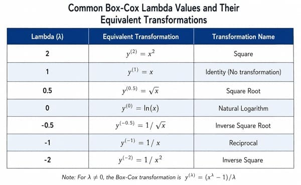
Analysts rarely calculate lambda by hand. Software finds the optimal value using maximum likelihood, then reports it. Several common lambda values correspond to transformations most practitioners already know:
| Lambda Value | Equivalent Transformation |
| 1.00 | No transformation needed |
| 0.50 | Square root |
| 0.33 | Cube root |
| 0.00 | Natural log |
| -0.50 | Reciprocal square root |
| -1.00 | Reciprocal (inverse) |
If the optimal lambda comes back close to a round number like these, many practitioners round to that simpler transformation. A rounded lambda is easier to explain to a team than a value like 0.42.
Also Read: 5 Simple Steps to Conducting a Non-Normal Capability Analysis in Minitab
A Real Six Sigma Example
A documented case from iSixSigma illustrates how this works in practice. A Green Belt was analyzing purchase order-generation cycle time data. The raw data failed a normality test, which meant a standard control chart would have used the wrong control limits.
The team ran a Box-Cox transformation and found an optimal lambda of 0.5, equivalent to a square root transformation. After transforming the data, a probability plot confirmed the data now fit a normal distribution. The Green Belt built a control chart on the transformed values and confirmed the process was stable, with all variation coming from common causes rather than a special cause.
One detail matters here. The transformed values themselves have no direct business meaning. The team still had to convert the control limits back into the original units before sharing results with stakeholders who needed to interpret real cycle times, not transformed ones.
How Six Sigma Applies the Box-Cox Transformation
The Box-Cox transformation plays a specific role inside DMAIC, mainly during the Measure and Analyze phases.
Define
The team identifies which process metric shows an unusual or skewed pattern, such as cycle time, defect counts, or a material property.
Measure
The team collects raw process data and runs a normality test, commonly the Anderson-Darling test. A low p-value signals the data does not fit a normal distribution.
Analyze
The team applies a Box-Cox transformation and lets the software search for the optimal lambda. A follow-up normality test on the transformed data confirms whether the fix worked.
Improve
The team builds capability studies or control charts using the transformed data, since these tools depend on the normality assumption to produce trustworthy limits.
Control
The team documents the lambda value used and keeps a clear record of how to convert transformed values, and control limits, back into original units for ongoing monitoring.
Limitations of the Box-Cox Transformation
The Box-Cox transformation works well, but it comes with real constraints teams should know before relying on it.
Requires strictly positive data. The method cannot handle zero or negative values. Teams with that kind of data typically add a small constant to every value first, or switch to the Yeo-Johnson transformation, which was built specifically to handle zero and negative numbers.
Reduces interpretability. A transformed value rarely means anything on its own to someone outside the analysis. Teams need to convert results back into original units before presenting them to stakeholders.
Assumes continuous data. The method fits continuous measurements far better than discrete counts or categorical data.
Is not always necessary. If the optimal lambda comes back close to 1, the data was already close to normal, and a transformation adds little value.
How to Run a Box-Cox Transformation Step by Step
Most Six Sigma practitioners run this transformation inside statistical software rather than by hand. The general steps stay consistent across platforms.
- Test the original data for normality. Run a test such as Anderson-Darling and check the p-value against your alpha level.
- Confirm the data is strictly positive. Add a small constant to every value if any are zero or negative.
- Run the Box-Cox transformation tool. In Minitab, this sits under Stat, then Control Charts, then Box-Cox Transformation. In SigmaXL, it sits under Data Manipulation.
- Review the suggested lambda value. Round it to a simpler value, such as 0.5 or 0, if the software allows and the difference is small.
- Re-test the transformed data for normality. Confirm the p-value now exceeds your alpha level.
- Build your control chart or capability study on the transformed data. Keep the lambda value on record for converting results back later.
Frequently Asked Questions: Box-Cox Transformation
Q: What is a Box-Cox transformation used for?
A: A Box-Cox transformation converts non-normal data into a shape that resembles a normal distribution. Analysts use it before running statistical tests, building control charts, or calculating process capability, since these tools assume the underlying data is normally distributed.
Q: Who invented the Box-Cox transformation?
A: Statisticians George E. P. Box and David R. Cox developed the method together. They published it in 1964 in a paper titled “An Analysis of Transformations” in the Journal of the Royal Statistical Society, Series B.
Q: What does lambda mean in a Box-Cox transformation?
A: Lambda is the power parameter that determines how the data gets transformed. A lambda of 1 means no real change, 0.5 corresponds to a square root, 0 corresponds to a natural log, and -1 corresponds to a reciprocal transformation.
Q: Can the Box-Cox transformation handle negative numbers?
A: No. The standard Box-Cox transformation requires strictly positive data. Data sets with zero or negative values typically need a constant added first, or a switch to the Yeo-Johnson transformation, which was designed to handle that kind of data directly.
Q: How do you choose the right lambda value?
A: Statistical software, such as Minitab or SigmaXL, tests a range of lambda values and selects the one that produces the best fit to a normal distribution using maximum likelihood. Analysts often round the result to a simpler, well-known value when the difference is small.
Q: Does a Box-Cox transformation change the meaning of my data?
A: Yes, in terms of scale. The transformed values do not carry the same direct meaning as the original units. Teams need to convert control limits or other results back into the original scale before sharing them with stakeholders.
Box-Cox Transformation Training in Six Sigma
Recognizing non-normal data, and knowing what to do about it, is a core skill for any Green Belt or Black Belt. Reading about the Box-Cox transformation helps, but applying it correctly inside a live DMAIC project is where the skill actually sticks.
At Six Sigma Development Solutions, our Green Belt and Black Belt training programs cover normality testing, data transformations, and the capability analysis that depends on them, using real process data as the working example.
We offer training in three formats:
- Onsite training: Delivered at your facility, using your own process data as the working example.
- Live virtual training: Instructor-led sessions delivered online with real-time interaction.
- Online training: Self-paced certification programs available at Green Belt and Black Belt levels.
Explore our Six Sigma training programs or contact our team to find the right program for your goals.
About Six Sigma Development Solutions, Inc.
Six Sigma Development Solutions, Inc. offers onsite, public, and virtual Lean Six Sigma certification training. We are an Accredited Training Organization by the IASSC (International Association of Six Sigma Certification). We offer Lean Six Sigma Green Belt, Black Belt, and Yellow Belt, as well as LEAN certifications.
Book a Call and Let us know how we can help meet your training needs.


