A histogram is one of the most basic tools in statistics. It helps visualize how data is distributed across different ranges. It provides an easy way to see the shape of the data. However, the distribution of data is not always uniform. It often has a skew, meaning that it leans to one side. Skewness can be either left (negative) or right (positive), depending on how the data is spread out.
When data is left-skewed, it means that there are a few data points that are much lower than the rest. These lower points pull the mean of the data towards the left. This results in a longer tail on the left side of the histogram.
Understanding left-skewed histograms is essential in fields like economics, psychology, and education. It can help make better decisions when interpreting data.
Table of contents
What Is a Left-Skewed Histogram?
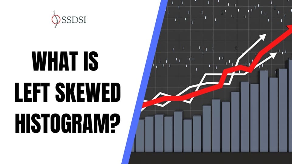
A left-skewed histogram, also known as a negatively skewed histogram, has a distinctive shape. In this type of histogram, the majority of the data points are concentrated on the right. The data tapers off to the left, creating a long tail. This means that most of the data values are higher, and fewer data points fall in the lower range.
When you look at a left-skewed histogram, the peak of the distribution is on the right. The tail, however, is stretched to the left, indicating that some data points are much smaller than the rest.
In these situations, the mean is usually smaller than the median because the low values pull the mean towards the left. The mode, or the most common value, is typically found on the right side of the distribution.
In comparison, a right-skewed histogram has a longer tail on the right side, with most values on the left. A symmetrical distribution, like a normal distribution, has data points spread evenly on both sides.
Key Features of Left-Skewed Histograms
A left-skewed histogram displays several distinctive features that set it apart from other types of distributions. Understanding these characteristics is crucial when interpreting data.
Mode, Median, and Mean in a Left-Skewed Distribution
The relationship between the mode, median, and mean in a left-skewed distribution is key to understanding the data:
Mode: The mode is the most frequent value in the dataset. In a left-skewed histogram, the mode tends to be found on the right side of the distribution, at the peak. This is because most data points are on the higher end of the scale.
Median: The median is the middle value when the data is arranged in ascending or descending order. In a left-skewed distribution, the median will fall between the mode and the mean but will be closer to the mode. The tail on the left side pulls the median toward the right, but it remains higher than the mean.
Mean: The mean is the arithmetic average of all data points. In a left-skewed histogram, the mean will always be lower than both the median and the mode. This occurs because extreme low values (outliers) on the left side have a greater influence on the mean than on the median or mode.
Position of the Peak and the Tail
The peak in a left-skewed histogram is on the right side, where the majority of data points are located. The tail, on the other hand, extends to the left. This tail represents a smaller number of data points that fall below the bulk of the data. The longer the left tail, the more pronounced the skewness.
In visual terms, a left-skewed histogram might appear “stretched out” toward the lower end of the data range. This characteristic is particularly important in statistics because it reveals that the data set includes a few extreme lower values that pull the overall distribution leftward.
Visual Differences in Left-Skewed Histograms
To spot a left-skewed histogram, look for the following:
Asymmetry: Most of the data points cluster on the right, with a gradual taper to the left.
Skewed tail: The left tail is noticeably longer than the right tail.
Unequal distribution: The data points on the left are sparse, while the bulk of the data is on the right.
These visual clues help analysts recognize skewness and take appropriate actions in their analysis.
Examples of Left-Skewed Distributions
Understanding where left-skewness appears in real-world data is crucial for applying statistical methods effectively. Below are some examples where left-skewed distributions are commonly found.
Income Distribution
Income distribution is one of the most cited examples of a left-skewed distribution. Most people earn average or above-average incomes, but a few individuals earn significantly lower incomes. This creates a distribution where the majority of the data is concentrated on the higher end, but the extreme lower values cause the distribution to skew to the left.
For example, in a company, most employees might earn decent salaries, but there could be a few employees who earn much lower wages. These lower-income individuals “pull” the mean down, resulting in a left-skewed histogram of salaries.
Retirement Age
The retirement age can also exhibit left skewness. While most individuals retire in their 60s or 70s, a small percentage of people retire earlier, often in their 40s or 50s. These early retirees contribute to the left tail of the distribution, creating a longer left side on the histogram.
The majority of people retiring later creates a peak on the right side, while the few early retirees cause the histogram to lean to the left. This is an example of a distribution where the data is mostly concentrated at the higher end but has a tail due to outliers.
Test Scores
Another example is test scores. In some cases, most students perform well on a test, but a few students may score significantly lower, especially if they were unprepared or missed the test. These lower scores create a left-skewed distribution.
The higher scores form the peak of the histogram, while the lower scores create the tail to the left.
In educational testing, this phenomenon can help identify areas where students may be struggling, or it can highlight the impact of outliers or anomalies in the dataset.
Implications of Left Skewness
Understanding the implications of left skewness is important for accurately interpreting data. Left-skewed distributions have a significant impact on how the central tendency measures (mean, median, and mode) are interpreted.
Relationship Between the Mean and Median
In a left-skewed distribution, the mean will always be less than the median. The reason is that the extremely low values, which form the left tail, “pull” the mean down. The median is not as sensitive to these extreme values and thus tends to be higher than the mean.
This relationship is essential when comparing different data sets. If a data set has a significant difference between the mean and median, it might indicate that the distribution is skewed, either left or right.
How does Skewness Affect Data Interpretation?
When analyzing skewed data, it’s important to recognize that the mean may not be the best measure of central tendency. In left-skewed data, the mean might give a false impression of where most of the data lies. In these cases, the median provides a better measure of the “typical” value.
For example, in salary data, if the mean is lower than the median, it could suggest that a few employees are earning very low wages, even though most employees earn higher salaries.
How Skewness Affects Decision-Making?
In decision-making, particularly in fields like economics, finance, and healthcare, recognizing skewness can be crucial. For example, if a business is analyzing customer spending, a left-skewed distribution might suggest that while most customers spend regularly, a few may spend far less. This could influence pricing strategies or marketing efforts aimed at increasing sales from lower-spending customers.
Statistical Methods for Analyzing Left-Skewed Data
When dealing with left-skewed data, certain statistical techniques can help to handle the skewness effectively.
Calculating Measures of Central Tendency
When analyzing left-skewed data, both the mean and median should be calculated. The mean will give you an idea of the overall data average, but the median is often more representative of the typical value. In cases of extreme skewness, the mode can also be helpful in identifying the most common value.
Using Transformations to Handle Skewness

In some cases, it may be necessary to “transform” skewed data to make it more symmetrical. Common transformations include:
- Log Transformation: Applying a logarithmic transformation can reduce skewness and make the distribution more normal.
- Square Root Transformation: This is useful when dealing with count data that is skewed.
- Box-Cox Transformation: A more advanced technique that can handle different types of skewness.
These transformations can make statistical analysis more reliable and improve the accuracy of predictive models.
Also See: Lean Six Sigma Certification Programs, Lubbock, Texas
Visualizing Left-Skewed Distributions
Visualizing a left-skewed distribution is essential for understanding its shape and nature. Histograms are the most common tool for visualizing skewed data. Other methods, like box plots or density plots, can also help reveal the skewness in the data.
Creating Histograms for Left-Skewed Data

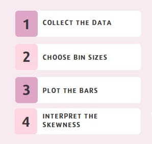
Histograms are simple to create and interpret. To create a histogram for left-skewed data, follow these steps:
- Collect the data: Gather the dataset that you want to analyze.
- Choose bin sizes: Divide the range of data into bins (intervals).
- Plot the bars: For each bin, count how many data points fall into that range and plot a bar.
- Interpret the skewness: Look for the left tail and determine how long it is.
Using Software Tools for Histogram Creation
There are several software tools available for creating histograms and analyzing skewed distributions. Tools like Excel, R, and Python (with libraries like Matplotlib or Seaborn) make it easy to generate and interpret histograms.
Final Words
A left-skewed histogram is a powerful tool for understanding the distribution of data. Recognizing skewness helps analysts interpret data more accurately and make informed decisions.
By examining the key features of left-skewed distributions, understanding the relationship between the mean, median, and mode, and applying the appropriate statistical methods, one can gain deeper insights into the dataset.
Whether you’re working with income data, test scores, or customer behaviours, understanding how to interpret and handle left-skewed data is an essential skill for anyone working with statistics.

About Six Sigma Development Solutions, Inc.
Six Sigma Development Solutions, Inc. offers onsite, public, and virtual Lean Six Sigma certification training. We are an Accredited Training Organization by the IASSC (International Association of Six Sigma Certification). We offer Lean Six Sigma Green Belt, Black Belt, and Yellow Belt, as well as LEAN certifications.
Book a Call and Let us know how we can help meet your training needs.


