Table of contents
What is a Chi-Squared Test?
The Chi-Squared Test is used to determine if an Attribute or Discrete “X” has an association with another Attribute or Discrete “Y.” The example below is a hypothesis (or an educated guess) that there is a relationship in Loan Default Rates between Bank Branches.
The Chi-Squared Test is intended to test how likely it is that an observed distribution of data is due to chance. The Chi-Squared Test is also called the “goodness of fit” statistic because it measures how well the observed distribution of data fits with the distribution that is expected if the variables are independent.
The Null and Alternative Hypotheses are:
- Ho = Variable A and Variable B are independent
- There is no effect on Defaulted Loans due to Bank Branches
- Ha = Variable A and Variable B are not independent
- There is an effect on Defaulted Loans due to Bank Branches
Chi-Squared Example
- A Bank has 200 Loan Approvals
- 100 Approvals from Branch “A”
- 100 Approvals from Branch “B”
- There are:
- 5 Loans defaulted from Branch “A”
- 9 Loans defaulted from Branch “B”
The Question: Is there a “real” difference in the default rates between the branches?
First, collect and summarize the data. This is the observed data.
Entered in Minitab as:

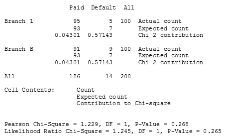
Analyzed as a Cross Tabulation and Chi-Square analysis the results are:

The expected values are calculated as follows:
r = Row total*(Column total / Grand total)
Example: 100*(186/200) = 93
The P value of 0.268 indicates that there is no relationship between branch and loan results. A p-value < 0.05 indicates a relationship may exist.
Next, the r values are investigated and the largest r value will have the most influence on the relationship.
Have you used a Chi-Squared Analysis in a Six Sigma Project? If so, can you give us a brief example of the analysis?


Some may be wondering, “So what does this analysis mean in practical terms?”
The results are telling you to “Fail to Reject the Null Hypothesis”.
Thus, even though the number of 5 defaults for Branch 1 and 9 defaults for Branch B seems to be a meaningful difference they aren’t different enough to support the Alternative Hypothesis.
Failing to Reject the Null Hypothesis with a Chi-Squared test for Independence and/or Proportions simply means the difference you are observing (e.g., in the default column) is just as likely to be a random chance as due to an assignable special cause.
Think of flipping 2 two-sided coins. The expectation (expected value) is equal distribution of heads and tails. Both coins could be “fairly” flipped (no trick coin and no gimmicks in the process. If each coin was flipped 100 times would you necessarily get an equal distribution of Heads and Tails..probably not. The coin toss wouldn’t be cited as having an assignable “Special Cause” driver until a specific threshold of improbability was met. When that improbability line is crossed the p-value will be less than the alpha value for the confidence level being tested at.
Therefore, if testing at 95% Confidence, the alpha value would be 0.05 (e.g., 5%). If the test Ch-Squared test result provided a p-value less than 0.05 (e.g., p=.001) then you would “Reject the Null Hypothesis”.
Rejecting the Null Hypothesis means your evidence from the test is strong enough to conclude the Alternative Hypothesis s more likely to be true. The difference in values CANNOT be explained away as random chance. The next step would be to investigate further and determine what Special Cause is driving a difference of Statistical Relevance (e.g., a “Rigged Coin” or a Gimmick in the process).
To learn more about this topic study how the “F” or Chi-Squared distribution Critical Value and respective Statistics are calculated. F Distribution and Chi-Squared Distribution analysis function the same way with the use of respective Degrees of Freedom tables to determine the Critical Value (the number of Rows and Columns determine the Critical Values in the table).
Meanwhile, an F or Chi-Squared “Statistic” is determined by the ratio of within variation (within subgroups) and between variations and is also impacted by the degrees of freedom. Reject the Null Hypothesis when the “Staistic” (e.g., F Statistic) is greater than the Critical Value (e.g., F Critical Value). Conversely, Fail to Reject the Null Hypothesis when the Statistic is less than the Critical Value.
NOTE: Magnitude matters. Susceptibility to a Type I Error (Producer’s Risk) or Type II Error (Consumer’s Risk) is greatest when the Test Statistic is close to the Critical Value. When this happens you should collect more data and run the test again.
Also, note that both the F Distribution and the Chi-Squared Distribution have the appearance of a long right-tailed Ski Slope. The distribution starts to look more normalized (approximating a flattened bell curve) when the number of degrees of freedom is substantially high (e.g., 20+ Degrees of Freedom).