
The chi-square distribution is a continuous probability distribution formed by summing the squares of independent standard normal random variables, and it is the reference distribution behind every chi-square test result.
Unlike the normal distribution, it can never take a negative value, which makes it right-skewed, especially at low degrees of freedom, where the curve looks like a steep backward “J” before flattening into something closer to a bell shape as degrees of freedom increase.
Most explanations stop at that shape description, but the detail that actually matters for practitioners is what the distribution is used for beyond hypothesis testing: it is the tool behind confidence intervals for variance and standard deviation, which makes it directly relevant to Six Sigma process capability work, not just categorical data testing. This guide covers the shape, the degrees of freedom relationship, where it differs from the chi-square test itself, and its overlooked role in variance estimation.
| Degrees of Freedom (df) | Shape | Peak Location | Approaches Normal? |
| 1 or 2 | Steep backward “J,” decays from zero | At zero | No |
| 3 to 9 | Hump-shaped, still right-skewed | At df − 2 | Slightly |
| 10 to 29 | More rounded, moderate skew | At df − 2 | Increasingly |
| 30 or more | Approximately symmetric, bell-shaped | Near the mean (df) | Yes |
Table of contents
Key Takeaways
- The chi-square distribution is the sum of squares of independent standard normal variables, which is why it can never be negative and why it is always right-skewed rather than symmetric like the normal distribution.
- Its shape is controlled entirely by one parameter, degrees of freedom (df). Low df produces a steep, heavily skewed curve; as df increases, the distribution gradually approaches the shape of a normal distribution.
- The mean of a chi-square distribution equals its degrees of freedom, and its variance equals twice the degrees of freedom, a relationship most glossary pages never mention despite it being useful for a quick sanity check on results.
- The chi-square distribution is not the same thing as the chi-square test. The distribution is the underlying probability model; the test is the specific hypothesis-testing procedure that uses that distribution to evaluate categorical data.
- Beyond categorical data testing, the chi-square distribution is the tool used to build confidence intervals for variance and standard deviation, a direct and often-overlooked connection to Six Sigma process capability analysis.
What Is the Chi-Square Distribution?
The chi-square distribution is a continuous probability distribution defined as the sum of the squares of k independent standard normal random variables, where k is the distribution’s single parameter, called degrees of freedom. Because every term being summed is a squared value, and squared numbers are never negative, the chi-square distribution itself can never take a negative value. This single mathematical fact explains nearly everything distinctive about its shape.

A chi-square distribution starts at zero and extends infinitely in the positive direction, with no left tail to speak of. That asymmetry is what makes it right-skewed: the distribution’s right tail stretches out further than a symmetric distribution would allow, while values pile up more densely near zero, especially at low degrees of freedom.
The chi-square distribution is technically a special case of the broader gamma distribution family, and it shows up as a building block inside other well-known distributions. The t-distribution and F-distribution, both heavily used elsewhere in Six Sigma hypothesis testing, are defined in part using the chi-square distribution, which makes understanding its shape useful well beyond chi-square tests themselves.

Public, Onsite, Virtual, and Online Six Sigma Certification Training!
- We are accredited by the IASSC.
- Live Public Training at 52 Sites.
- Live Virtual Training.
- Onsite Training (at your organization).
- Interactive Online (self-paced) training,
How Degrees of Freedom Shape the Curve
This is the section most competing explanations gloss over with a single sentence, and it is worth understanding in more depth, because the shape has real practical consequences for interpreting results.
At 1 or 2 degrees of freedom, the chi-square distribution looks like a steep, backward “J”: it starts at its highest point right at zero and decays rapidly, meaning that small chi-square values are highly likely and large ones become rare very quickly. At 3 or more degrees of freedom, the shape becomes hump-shaped rather than monotonically decreasing, with the peak of the curve occurring at df − 2.
A chi-square distribution with 10 degrees of freedom, for example, peaks at 8, not at 10, a detail worth knowing since it is easy to assume the peak and the mean are the same point, and they are not.
As degrees of freedom continue to increase, the distribution’s skew gradually decreases and the curve becomes more symmetric, eventually approximating a normal distribution once degrees of freedom reach roughly 30 or higher. This matters practically: at low degrees of freedom, treating chi-square results with normal-distribution intuition, assuming symmetry around the mean, for instance, produces meaningfully wrong conclusions.
At high degrees of freedom, that same normal-distribution intuition becomes a reasonably safe approximation.
The distribution’s mean equals its degrees of freedom, and its variance equals twice its degrees of freedom. A chi-square distribution with 6 degrees of freedom has a mean of 6 and a variance of 12. This relationship offers a fast sanity check: if a calculated chi-square statistic falls wildly outside a range consistent with its degrees of freedom, it is worth double-checking the calculation before drawing conclusions.
Also Read: Data Distributions in Six Sigma: Types, How to Identify Them, and Why They Matter
Chi-Square Distribution vs. Chi-Square Test: A Distinction Worth Making Precisely
These two terms get used almost interchangeably online, and the confusion causes real problems for anyone trying to actually understand what a test result means.
The chi-square distribution is a mathematical probability model, a specific shape of curve defined by degrees of freedom, that describes how a particular type of statistic behaves under certain assumptions. The chi-square test is a hypothesis-testing procedure, either a goodness of fit test or a test of independence, that calculates a test statistic from observed data and compares that statistic against the chi-square distribution to determine statistical significance.
Put simply: the distribution is the ruler, and the test is the specific act of using that ruler to measure something. A chi-square test statistic only means anything because the chi-square distribution describes the range of values that statistic would take purely by chance, assuming the null hypothesis is true. Without the distribution, there would be no way to convert a raw chi-square statistic into a meaningful p-value or critical value.
The Connection Most Glossaries Miss: Confidence Intervals for Variance
Nearly every basic explanation of the chi-square distribution focuses exclusively on its role in hypothesis testing for categorical data. That is only half the story, and it is the less useful half for Six Sigma practitioners specifically working on process capability.
According to statistical guidance on confidence intervals, the chi-square distribution is the standard tool used to build a confidence interval around a population variance or standard deviation, using degrees of freedom equal to sample size minus 1. Because the chi-square distribution is asymmetric, this calculation requires two separate critical values, a lower and an upper bound, drawn from different points on the distribution, unlike the single symmetric margin of error used for a confidence interval on a mean.
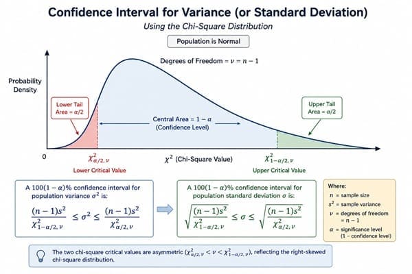
This connection matters directly to Six Sigma work. Process capability indices like Cp and Cpk depend on an accurate estimate of process standard deviation.
A team that only has a sample estimate of variability, not the true population value, can use the chi-square distribution to construct a confidence interval around that standard deviation, giving a defensible range instead of treating a single sample estimate as if it were certain. This is a materially different and more rigorous application of the chi-square distribution than categorical data testing, and it rarely appears in general-purpose explanations of the topic.
Where the Chi-Square Distribution Shows Up in a Six Sigma Project
- Chi-square tests in the Analyze phase. Every chi-square test of independence or goodness of fit relies on the chi-square distribution to determine statistical significance, most commonly when screening categorical input variables against a categorical outcome.
- Confidence intervals for standard deviation in capability studies. When a Black Belt needs to express uncertainty around a process’s estimated variability, rather than reporting a single Cpk number as if it were exact, the chi-square distribution provides the statistical basis for that range.
- ANOVA and variance comparison tools. The chi-square distribution also underlies certain tests for comparing variances across groups, relevant when a team is checking whether variation differs meaningfully between shifts, machines, or suppliers before pooling data together.
- As a building block for the F-distribution. Since the F-distribution used in ANOVA is defined using two chi-square distributions, understanding chi-square’s shape helps make sense of why ANOVA results behave the way they do at different sample sizes.
Also Read: Bimodal Distribution: Definition, Causes, and What It Means for Six Sigma
Real Examples of the Chi-Square Distribution in Practice
Manufacturing: Estimating True Process Variability
A Black Belt measures wall thickness on 25 injection-molded parts and calculates a sample standard deviation. Rather than reporting that single number as the definitive process variability, the team uses the chi-square distribution with 24 degrees of freedom to build a 95 percent confidence interval around the true population standard deviation, giving leadership an honest range instead of false precision.
Healthcare: Comparing Variation in Wait Times Across Clinics
A hospital system wants to know whether wait time variability differs meaningfully across three clinic locations, not just whether average wait times differ. Because comparing variances relies on chi-square-based statistical tools, this becomes a natural extension of variance-focused chi-square applications rather than a simple mean comparison.
Quality Engineering: Validating a Measurement System’s Consistency
A quality engineer wants a confidence interval around the standard deviation of repeated measurements taken by a single gauge, to understand how much of a product’s measured variability is coming from the gauge itself versus the actual parts. The chi-square distribution provides the statistical foundation for that interval.
Common Mistakes When Working With the Chi-Square Distribution
- Assuming the distribution is symmetric like the normal distribution. At low degrees of freedom especially, this assumption produces meaningfully wrong intervals and conclusions.
- Confusing the distribution’s peak with its mean. The peak of a chi-square curve with more than 2 degrees of freedom sits at df − 2, not at df, which is the actual mean.
- Treating chi-square distribution and chi-square test as synonyms. The distribution is the mathematical model; the test is the specific procedure applied to categorical data using that model.
- Ignoring the distribution’s role in variance estimation. Limiting chi-square’s relevance to categorical data testing misses one of its most practically useful Six Sigma applications: building honest confidence intervals around process variability.
- Using normal-distribution intuition at low degrees of freedom. The chi-square distribution only starts resembling a normal distribution once degrees of freedom reach roughly 30; below that, its skew is significant enough to change conclusions.
Frequently Asked Questions on Chi-Square Distribution
Why is the chi-square distribution always right-skewed?
Because it is defined as the sum of squared standard normal variables, which can never be negative. This forces the distribution to start at zero and extend only in the positive direction, producing a longer right tail than a symmetric distribution would have.
What is the difference between the chi-square distribution and the chi-square test?
The chi-square distribution is the underlying mathematical probability model. The chi-square test is a specific hypothesis-testing procedure, either goodness of fit or test of independence, that uses that distribution to evaluate categorical data and determine statistical significance.
How do degrees of freedom affect the shape of the chi-square distribution?
At low degrees of freedom, the distribution is steeply right-skewed, resembling a backward “J.” As degrees of freedom increase, the curve becomes more symmetric and eventually approximates a normal distribution once degrees of freedom reach roughly 30 or more.
How is the chi-square distribution used outside of categorical data testing?
It is the statistical foundation for building confidence intervals around population variance and standard deviation, which makes it directly relevant to Six Sigma process capability studies, not just chi-square tests on categorical data.
What is the mean and variance of a chi-square distribution?
The mean equals the degrees of freedom, and the variance equals twice the degrees of freedom. A chi-square distribution with 6 degrees of freedom, for example, has a mean of 6 and a variance of 12.
Final Words
The chi-square distribution is easy to reduce to “the thing behind the chi-square test,” but that undersells what it actually does. Its right-skewed shape, its degrees-of-freedom relationship, and its lesser-known role in building honest confidence intervals around process variability all matter directly to how a Six Sigma practitioner interprets uncertainty in real project data.
Six Sigma Development Solutions Inc. teaches the chi-square distribution, confidence intervals for variance, and the full statistical toolkit behind capability analysis through onsite, live virtual, public, and online formats. Our Green Belt and Black Belt certification courses work through real variability data, not just theory. View our upcoming Green Belt and Black Belt training schedule and get $500 off your next class.
About Six Sigma Development Solutions, Inc.
Six Sigma Development Solutions, Inc. offers onsite, public, and virtual Lean Six Sigma certification training. We are an Accredited Training Organization by the IASSC (International Association of Six Sigma Certification). We offer Lean Six Sigma Green Belt, Black Belt, and Yellow Belt, as well as LEAN certifications.
Book a Call and Let us know how we can help meet your training needs.


