Survival Analysis

Survival analysis is a statistical method focused on analyzing and interpreting survival outcomes. These outcomes often measure the time until a specific event occurs, such as death, disease progression, or equipment failure. This method is important across various fields such as medicine, engineering, and social sciences, offering insights into time-to-event data.

What is Survival Analysis?

Survival analysis refers to a set of statistical methods designed to analyze time-to-event data. This branch of statistics helps us understand the timing of specific events, referred to as “failures.” To be more precise, the term “failure” in survival analysis denotes the event of interest, which could be anything from death to recovery from a disease, depending on the context.

For example, survival analysis is commonly applied in medical research to study patient survival post-surgery, in veterinary science. This is to examine the time cows take to conceive after calving, or in epidemiology to investigate the time a farm takes to report its first case of an exotic disease.

Key Concepts in Survival Analysis

Survival Time (T):
Survival time refers to the time duration from a defined starting point to an event of interest. The event can be terminal (e.g., death) or non-terminal (e.g., disease relapse).
Examples:

• Time from cancer diagnosis to death.
• Time from vaccine administration to infection.
• Time from treatment initiation to disease progression.

Types of Survival Time Data:

• Discrete: Specific intervals (e.g., years, days).
• Continuous: Measured precisely (e.g., hours, seconds).

Survival analysis predominantly deals with continuous data.

Key Components of Survival Analysis

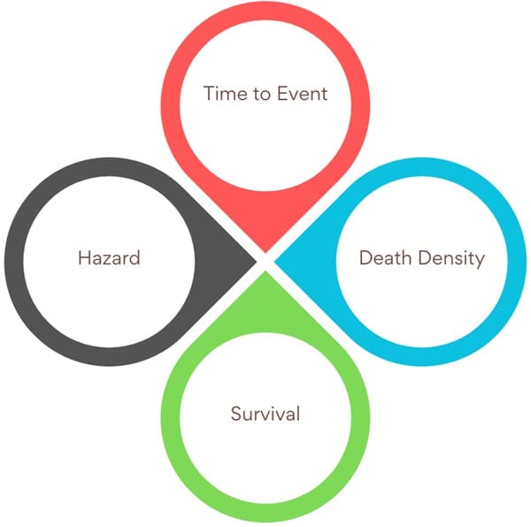
1. Time to Event
   The primary variable in survival analysis is the duration until the occurrence of the event of interest, termed “survival time.” Understanding this duration is the key to many real-world applications. Examples:
   • The survival duration of patients post-surgery.
   • The time taken for cows to conceive after calving.
   • The period a farm remains free of a specific disease.
2. Death Density
   At the time of analyzing the time taken for an event like death to occur, we can use a frequency histogram to visualize the number of events as a function of time. The curve derived from this histogram is called the death density function f(t). If the total area under this curve equals 1, the cumulative area up to a specific time t represents the proportion of the population that has experienced the event by that time. This proportion is known as the cumulative death distribution function F(t).
3. Survival
   The area under the death density function beyond time t represents the proportion of individuals who have survived up to time t. This proportion, denoted as S(t), forms the basis of the survival curve, a stepwise graph used to visualize survival data. At the start (t=0), the survival probability is 1 (or 100%), decreasing as events occur.
4. Hazard
   The hazard function quantifies the instantaneous risk of an event at a specific time. It represents the probability that an individual who has survived until time t will experience the event in the next infinitesimal time interval. Mathematically, it is the ratio of the number of events occurring between t and t+Δt to the population at risk at t. This function is also known as the failure rate or instantaneous death rate.

Censoring in Survival Analysis

In survival studies, not all individuals experience the event of interest during the observation period. In this case, their exact survival time remains unknown. These incomplete observations are referred to as censored data. Survival analysis accommodates this data to maximize the use of available information.

Types of Censoring

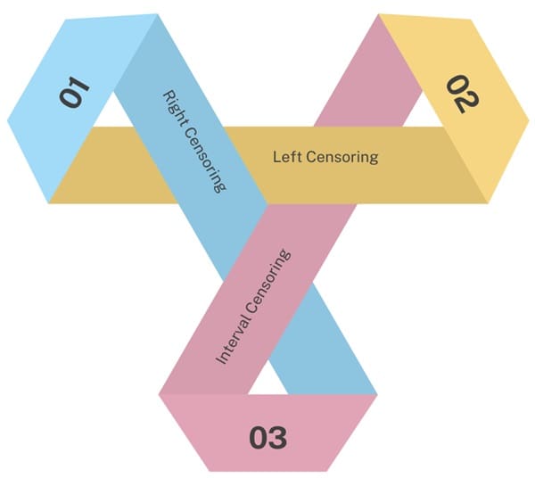
1. Right Censoring: It occurs when the event is known to happen after the observation period. For instance, a patient is alive at the end of a study but could pass away later.
2. Left Censoring: This happens when the event occurs before the observation begins. For example, if a study tracks cows post-calving but some cows have already conceived before the start, they are left censored.
3. Interval Censoring: It takes place when the event happens within a known time interval, but the exact time is uncertain. For example, testing cows every six months for seroconversion in a disease study.

Truncation:
Truncation differs from censoring as it represents periods where the event of interest cannot possibly occur.

• Left Truncation: The event cannot occur before the subject enters the study.
• Right Truncation: The event cannot occur after a subject leaves the study.

Non-Parametric Methods in Survival Analysis

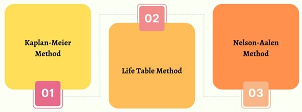
These methods are often preferred when the data does not fit theoretical distributions. These techniques provide flexible ways to describe survival data without assuming specific distributions. Three common non-parametric methods are:

1. Kaplan-Meier Method
   The Kaplan-Meier estimator is widely used for individual survival times. It calculates the probability of survival over time by multiplying conditional probabilities for each time interval. This method assumes that the censoring process is independent of the event occurrence.
2. Life Table Method
   It is alternatively known as the actuarial method. This approach groups survival times into intervals, making it suitable for large datasets. It approximates survival probabilities while assuming events and censoring occur uniformly within each interval.
3. Nelson-Aalen Method
   This method estimates cumulative hazard rates directly. It is often used in conjunction with the Kaplan-Meier method to provide a detailed understanding of the underlying hazard process.

Also See: Lean Six Sigma Certification Programs, Chandler, Arizona

Applications of Survival Analysis

Survival analysis is versatile and finds applications across various fields:

1. Medicine: Studying the survival rates of patients after treatments or surgeries.
2. Veterinary Science: Analyzing conception times in livestock.
3. Epidemiology: Tracking the time to disease outbreaks in populations or farms.
4. Manufacturing: Assessing product reliability and failure times in quality control.
5. Social Sciences: Evaluating the time until specific life events, such as marriage or employment.

Strengths of Survival Analysis

1. Handling Censored Data: Unlike many statistical methods, survival analysis incorporates censored observations, ensuring no data is wasted.
2. Flexibility: This can be applied to diverse datasets, regardless of whether the time to event follows a standard distribution.
3. Insightful Visualization: Survival curves and hazard functions offer clear insights into time-dependent processes.
   Advanced Topics in Survival Analysis
4. Score and Fisher Information: The log-likelihood function captures the probability of observing the data given the parameters. Its derivative, known as the score, is used to find the MLE. The second derivative provides the Fisher Information, which helps estimate parameter variances.
5. Multivariate Survival Analysis: For models with multiple parameters, the score becomes a vector, and the Hessian matrix (second derivative matrix) is used to solve for parameter estimates.

Practical Challenges in Survival Analysis

Censoring Complexity: Dealing with censored data requires sophisticated techniques to ensure accurate parameter estimation and prediction.

Assumption of Distribution: The choice of distribution (exponential, Weibull, etc.) significantly impacts results. Incorrect assumptions can lead to biased estimates.

Treatment Effects: In clinical trials, censoring may correlate with treatment effects, complicating the analysis. For example, patients responding well to treatment may remain in the study longer, introducing bias.

Visualizing Survival Data

Survival analysis often includes graphical representations such as:

Survival Curves:
These curves depict the proportion of individuals surviving over time, helping compare treatment groups.

Hazard Plots:
Hazard plots show risk patterns and identify critical periods of high risk.

Cumulative Hazard Graphs:
These graphs illustrate accumulated risk over time, providing insights into long-term trends.

Final Words

Survival analysis is a powerful tool for understanding time-to-event data. Its ability to incorporate censored data and model time-dependent phenomena makes it indispensable in medical research, epidemiology, and beyond. By providing insights into survival times, hazard rates, and cumulative risks, survival analysis aids decision-making and advances our understanding of dynamic processes.

Related Articles

• t-Distribution
• How To: One Sample T Test
• Bimodal Distribution
• What is a Kaizen Event?
• Confidence Interval