
You measure a sample of parts and find the average diameter is 10.2mm. But how reliable is that number? Does it describe the whole process, or just the 30 parts you happened to measure?
This is exactly the problem a confidence interval solves.
A confidence interval (CI) is a range of values that, with a stated level of probability, contains the true population parameter you are trying to estimate. Instead of a single point estimate — “the average is 10.2mm” — a confidence interval gives you a range: “we are 95% confident the true average falls between 10.05mm and 10.35mm.”
In Lean Six Sigma, you almost never have access to every data point in a population. You work with samples. And any time you work with samples, there is uncertainty. A confidence interval makes that uncertainty visible and measurable, which is far better than ignoring it.
This article explains what a confidence interval is, how to interpret it correctly, where it fits in DMAIC, and the most common mistakes practitioners make when using it.
Table of contents
What a Confidence Interval Actually Means?
The phrasing “95% confident” trips up a lot of people. It does not mean there is a 95% chance the true value is inside this specific interval. The true value either is or is not in any given interval — there is no probability about it.
What the 95% refers to is the long-run method. If you repeated your sampling process many times and built a confidence interval from each sample, roughly 95% of those intervals would contain the true population parameter.
In practice, what this means for a Six Sigma practitioner is straightforward: a 95% confidence interval calculated from a representative sample is a reliable estimate of where the true process parameter sits. The wider the interval, the more uncertainty in your estimate. The narrower, the more precise.
Three things affect how wide or narrow a confidence interval is:
Sample size: Larger samples produce narrower intervals. Doubling your sample size reduces the margin of error, giving you a tighter, more useful estimate.
Process variability: High variation in the process produces wider intervals. Reducing process variation — one of the core goals of Six Sigma — also tightens your confidence intervals.
Confidence level chosen: A 99% confidence interval is wider than a 95% interval, which is wider than a 90% interval. Higher confidence comes at the cost of precision. The most common level used in Six Sigma work is 95%.

Public, Onsite, Virtual, and Online Six Sigma Certification Training!
- We are accredited by the IASSC.
- Live Public Training at 52 Sites.
- Live Virtual Training.
- Onsite Training (at your organization).
- Interactive Online (self-paced) training,
Confidence Level vs. Significance Level
These two terms are closely related, and mixing them up causes real errors in analysis.
The confidence level is the probability that your interval contains the true parameter. A 95% confidence level means you are willing to accept a 5% chance your interval misses the true value.
The significance level (alpha, α) is that 5% — the risk you are willing to accept that you will incorrectly conclude a difference exists when it does not. In hypothesis testing, the standard alpha is 0.05 (5%).
The relationship is simple: confidence level = 1 − alpha.
A 95% confidence interval corresponds to a 5% significance level. A 99% confidence interval corresponds to a 1% significance level.
When you see a confidence interval that does not overlap zero (for a difference between two groups) or does not include a benchmark value, that is usually telling you the same thing a hypothesis test would tell you: the result is statistically significant at the corresponding alpha level.
How Confidence Intervals Are Used in DMAIC
Confidence intervals appear throughout a Six Sigma DMAIC project. Here is where they matter most.
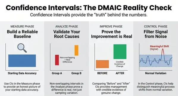
Measure Phase: Establishing a Reliable Baseline
Before you can improve a process, you need an accurate baseline. A single mean calculated from a small sample might not represent the process accurately. Reporting your baseline with a confidence interval — “the average defect rate is 8.2%, with a 95% CI of 6.9% to 9.5%” — gives stakeholders a more honest picture of what you actually know.
This also forces honesty about sample size. If your confidence interval is very wide, it is a signal that you need more data before drawing conclusions.
Analyze Phase: Validating Root Causes
In the Analyze phase, confidence intervals help you confirm whether a suspected root cause is genuinely affecting the output, or whether the observed difference could be explained by random sampling variation.
For example: if you suspect Machine A produces more defects than Machine B, you can compare the two defect rates with confidence intervals. If those intervals do not overlap, that is evidence the difference is real. If they do overlap significantly, the difference may just be noise.
This is closely connected to hypothesis testing. Confidence intervals and p-values are two ways of looking at the same question: is this difference statistically meaningful?
Improve Phase: Confirming the Improvement Is Real
After you implement a solution, you need to show the improvement is genuine — not just random variation in the data. A confidence interval on the after-improvement data that does not overlap with the before-improvement baseline is strong evidence that a real change occurred.
This matters for management sign-off. “Defects went from 8.2% to 3.1%” is a claim. “Defects went from 8.2% (95% CI: 6.9–9.5%) to 3.1% (95% CI: 2.4–3.8%)” is evidence. The non-overlapping intervals tell a clear, credible story.
Control Phase: Monitoring Process Performance
In the Control phase, confidence intervals help set monitoring thresholds. When a process metric drifts outside an expected range, a confidence interval helps distinguish a meaningful shift from normal variation. This supports more intelligent control chart responses — acting on real signals while ignoring noise.
Reading a Confidence Interval: A Practical Example
Suppose a Six Sigma team is working to reduce order processing time. They sample 50 orders before the improvement and calculate:
- Mean processing time: 4.8 days
- 95% Confidence Interval: 4.2 to 5.4 days
After the improvement, they sample another 50 orders:
- Mean processing time: 3.1 days
- 95% Confidence Interval: 2.7 to 3.5 days
The two intervals do not overlap. The highest value of the post-improvement CI (3.5 days) is well below the lowest value of the pre-improvement CI (4.2 days). This is strong statistical evidence that the improvement produced a real reduction in processing time — not just a lucky sample.
If the intervals had overlapped, the team would need more data or a formal hypothesis test before claiming the improvement was statistically proven.
Also Read: Survival Analysis: Predict Time-to-Event with Confidence
90%, 95%, or 99%: How to Choose Your Confidence Level
The most common default in Six Sigma is 95%. It strikes a practical balance between confidence and precision.
Use 90% when the cost of being wrong is low and you want a tighter interval — exploratory analysis or initial screening, for example.
Use 95% as your standard working level for most DMAIC analysis, root cause validation, and improvement confirmation.
Use 99% when the stakes are high — safety-critical processes, medical or pharmaceutical applications, or situations where a false positive would have serious consequences.
One caution: choosing a higher confidence level because you want to appear more rigorous, without a corresponding increase in sample size, just gives you a wider interval that is less useful. Confidence level and sample size need to be planned together before data collection, not adjusted afterward.
Common Mistakes When Using Confidence Intervals
Saying “there is a 95% chance the true value is in this interval.” This is the most widespread misstatement. The true value is fixed — it does not have a probability of being somewhere. The 95% refers to the method, not the specific interval.
Ignoring confidence intervals entirely and reporting only point estimates. A mean without an interval hides how much uncertainty is in the estimate. In Six Sigma work, this often leads to overconfidence in baseline measurements or improvement claims.
Concluding that overlapping intervals mean no significant difference. Overlapping confidence intervals do not automatically mean the two groups are the same. Interval overlap is a visual guide, not a formal test. For a definitive answer, run the appropriate hypothesis test.
Confusing statistical significance with practical significance. A confidence interval that does not include zero tells you a difference is statistically real. It does not tell you whether the difference is large enough to matter to the business. A 0.05-day reduction in processing time might be statistically significant with a large enough sample, but operationally meaningless. Always interpret CIs alongside practical context.
Using confidence intervals on unstable processes. Just as capability analysis requires a stable process, so does meaningful confidence interval calculation. If your process is erratic, your sample may not represent steady-state behavior, making the interval misleading.
Confidence Intervals and Sample Size Planning
One of the most practical uses of confidence interval theory is planning your data collection before a project begins.
If you know how wide a confidence interval you need (how precise your estimate must be) and what the approximate process variability is, you can calculate the minimum sample size required to achieve that precision.
This prevents one of the most common Six Sigma project delays: collecting data, calculating an interval, finding it is too wide to draw conclusions, and having to go back for more samples.
The formula for the required sample size for a mean (with known standard deviation) is:
n = (Z × σ / E)²
Where:
- Z = the Z-score for your chosen confidence level (1.96 for 95%, 2.576 for 99%)
- σ = the estimated process standard deviation
- E = the desired margin of error (half the width of the CI)
If your standard deviation is not known in advance, use a small pilot sample to estimate it, then calculate the full sample size needed.
Also Read: Confidence Level
Learn Statistical Tools Including Confidence Intervals in Our Training
Confidence intervals are taught as part of the statistical foundation in both our Green Belt and Black Belt programs. You will not just learn the formula — you will work through real examples, use statistical software, and understand when and how to apply CIs in an actual DMAIC project.
At Six Sigma Development Solutions Inc., we offer training in three formats:
- Onsite training at your facility, with examples drawn from your own processes
- Live virtual classroom with a live instructor, real-time Q&A, and structured projects
- Online self-paced certification you can complete on your own schedule
Our Green Belt program covers confidence intervals, hypothesis testing, sample size planning, and the full Analyze phase statistical toolkit. Our Black Belt program goes deeper into advanced hypothesis testing, regression, and design of experiments.
About Six Sigma Development Solutions, Inc.
Six Sigma Development Solutions, Inc. offers onsite, public, and virtual Lean Six Sigma certification training. We are an Accredited Training Organization by the IASSC (International Association of Six Sigma Certification). We offer Lean Six Sigma Green Belt, Black Belt, and Yellow Belt, as well as LEAN certifications.
Book a Call and Let us know how we can help meet your training needs.


