Residual Analysis

Residual analysis plays a critical role in assessing the quality of a regression model after fitting it to data. After performing regression, it’s important to evaluate the model’s adequacy by examining how well it captures the underlying relationship between variables.

Residual analysis helps us verify that the assumptions behind the regression model hold true, which is essential for making valid inferences. This article explores the concept of residuals, outlines their properties, and demonstrates how to use them to identify potential issues in regression models.

What are Residuals?

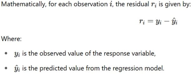
Residuals are the differences between observed and predicted values of the response variable in a regression model. They are calculated by subtracting the predicted value (obtained from the regression model) from the observed value.

Residuals help identify how well the model fits the data. Specifically, they highlight the discrepancy between the actual data points and the model’s predictions.

Residuals are used to evaluate several assumptions underlying the regression model. These assumptions include linearity, constant variance (homoscedasticity), and normality of errors. If the residuals behave unexpectedly, they indicate that one or more assumptions are violated and suggest that the model may not be appropriate for the data.

Why Do We Need Residual Analysis?

Residual analysis is crucial for validating the assumptions of regression analysis and improving the model. The main goal is to check if the regression model fits the data well and if the underlying assumptions hold true. These assumptions are as follows:

1. Zero Mean of Errors: The errors ϵi\epsilon_iϵi​ should have a mean of zero.
2. Constant Variance of Errors (Homoscedasticity): The variance of errors should be constant across all levels of the independent variables.
3. No Autocorrelation: Errors for different observations should not be correlated.
4. Normality of Errors: The errors should follow a normal distribution.

Violations of any of these assumptions can lead to misleading results in regression analysis. Residual analysis helps to detect such violations and guide corrective actions, such as transforming variables, using different modeling techniques, or adding new variables.

Also Read: Time Series Analysis

Difference Between Errors and Residuals

It’s important to differentiate between residuals and errors in regression analysis. While both concepts refer to differences between observed and predicted values, they are not the same:

• Error terms (denoted as ϵi\epsilon_iϵi​) represent the difference between the observed value and the true underlying value of the response variable. These error terms are unobservable because we cannot know the true underlying model perfectly.
• Residuals (denoted as rir_iri​) are the differences between the observed and predicted values of the response variable based on the fitted model. Unlike error terms, residuals can be calculated directly from the data.

Although residuals approximate the error terms, they differ because we can calculate residuals from the data, whereas error terms are theoretical quantities that we cannot measure directly.

Role of Residuals in Model Diagnostics

The primary purpose of residual analysis is to check if the underlying assumptions of the regression model are valid. The following are key assumptions to verify:

1. Linearity: The relationship between the response and explanatory variables should be approximately linear.
2. Homoscedasticity: The variance of the residuals should remain constant across all levels of the explanatory variables.
3. Normality: The residuals should follow a normal distribution, especially for statistical inference and hypothesis testing to be valid.
4. Independence: The residuals should be uncorrelated with each other, meaning that the errors at one observation should not provide any information about errors at another observation.

Model Adequacy Checking Through Residual Analysis

After fitting a regression model, we can perform various diagnostic checks to assess whether the assumptions hold true. Residual analysis offers a way to detect any potential problems. Let’s break down the essential steps involved in this analysis:

1. Examine Linearity: In both simple and multiple regression models, one key assumption is that the relationship between the response and explanatory variables should be linear. This can be checked by plotting residuals against the fitted values or explanatory variables. If the residuals show any pattern (such as a curved shape), it indicates a violation of the linearity assumption.
2. Check for Homoscedasticity: Homoscedasticity refers to the assumption that the residuals have constant variance across all levels of the explanatory variables. If the residuals fan out or contract as the fitted values increase, it suggests heteroscedasticity (i.e., non-constant variance), which violates this assumption.
3. Check for Normality: Residuals should ideally follow a normal distribution for the regression model’s statistical tests to be reliable. This can be assessed using graphical methods such as normal probability plots (Q-Q plots) or histograms of residuals. If the residuals deviate significantly from normality, it may indicate a problem with the model.
4. Independence of Residuals: You can check the independence of residuals by plotting them against time or another relevant variable. If you observe correlation among the residuals, it suggests that the model may be missing an important variable or feature, which could lead to misleading conclusions.

Types of Residual Plots

Several types of plots are commonly used in residual analysis to evaluate the assumptions:

1. Residuals vs. Fitted Values Plot: This plot helps assess the linearity and homoscedasticity assumptions. If the residuals appear randomly scattered with no discernible pattern, the assumptions are likely valid. However, if there is a systematic pattern (such as a funnel shape or curve), it suggests a problem with the model.
2. Normal Q-Q Plot: A normal quantile-quantile plot (Q-Q plot) compares the distribution of residuals to a normal distribution. If the points on the plot form a straight line, it indicates that the residuals follow an approximately normal distribution.
3. Scale-Location Plot: This plot helps check for homoscedasticity by showing the residuals’ spread as a function of the fitted values. If the residuals are uniformly spread, the assumption of constant variance is likely satisfied.
4. Leverage vs. Residuals Plot: This plot helps identify influential data points that might disproportionately affect the model’s fit. Points with high leverage and large residuals should be carefully examined.

Also Read: Residuals

Interpreting Residual Plots

1. Linearity: If the residuals show a pattern or trend (such as a curve), the linearity assumption may be violated. For instance, a fan-shaped plot suggests that the variance of residuals is not constant (i.e., heteroscedasticity), which violates the homoscedasticity assumption.
2. Homoscedasticity: Ideally, the residuals should scatter evenly around zero with no specific shape. If the spread of residuals increases or decreases with fitted values, the assumption of homoscedasticity is violated.
3. Normality: The normal Q-Q plot should ideally show points close to a straight line. When the points significantly deviate from this line, they suggest that the residuals are not normally distributed, which may impact the statistical inference drawn from the model.
4. Independence: Autocorrelation or clustering of residuals can indicate a problem with the model, suggesting that residuals from one observation are influencing others.

Residual Plots and Patterns

These plots are valuable tools for identifying problems in the regression model. Let’s explore common patterns that can appear in residual plots and their implications:

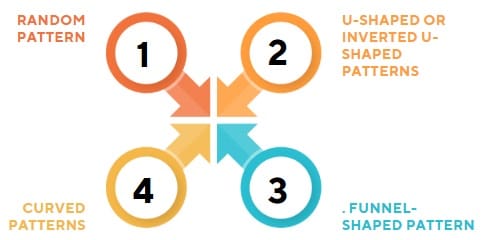
1. Random Pattern:

When the residuals are randomly scattered around zero without a clear pattern, they indicate that the model is appropriate and that the underlying assumptions are likely satisfied. This is the ideal scenario for linear regression.

2. U-Shaped or Inverted U-Shaped Patterns:

If the residuals form a U-shape or inverted U-shape, it indicates that the model may be missing a quadratic term or a higher-order relationship. This suggests that a linear model is not suitable, and you might need to include additional terms or transform the variables.

3. Funnel-Shaped Pattern:

A funnel shape, where the residuals spread out or contract as the predicted values increase, indicates heteroscedasticity. This suggests that the variance of the errors is not constant, which can lead to inefficient parameter estimates. One solution is to apply weighted least squares regression or transform the dependent variable.

4. Curved Patterns:

Curved patterns in residual plots suggest nonlinearity in the relationship between the independent and dependent variables. This indicates that a linear regression model may not be appropriate, and you might need to incorporate nonlinear terms, such as polynomials or interaction effects.

Also Read: Right Skewed Histogram

Computation of Residuals and Scaled Residuals

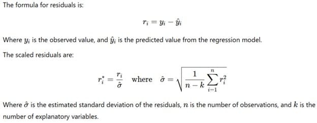
In order to perform residual analysis, it’s essential to calculate residuals and scaled residuals. The residual for each observation is simply the difference between the observed value and the predicted value. For a more refined analysis, scaled residuals are sometimes used.

We compute scaled residuals by dividing the residuals by an estimate of their standard deviation, which helps identify outliers more effectively.

How to Check for Assumptions Using Residuals?

You can check the assumptions mentioned above using residual plots and diagnostic tools. Residual plots graphically represent the residuals by plotting them against various variables, such as predicted values, observed values, or independent variables. Let’s go through each of the key checks:

1. Zero Mean of Errors:

One way to check for zero mean is by plotting the residuals against the predicted values. Ideally, the residuals should be scattered randomly around zero, indicating that the errors have zero mean. If there is a systematic trend, it could suggest that the model is missing a relevant variable or that a nonlinear relationship exists.

2. Constant Variance of Errors (Homoscedasticity):

Constant variance of the errors is essential for reliable regression estimates. To check for homoscedasticity, we can plot the residuals against the predicted values. If the variance of the residuals increases or decreases as the predicted value increases, you are observing heteroscedasticity, which violates the assumption of constant variance.

For example, if the residuals form a funnel shape that opens outward as the predicted value increases, it indicates increasing variance (heteroscedasticity). Conversely, if the funnel shape opens inward, it suggests decreasing variance.

3. No Autocorrelation:

Autocorrelation occurs when the residuals for one observation are correlated with the residuals for another observation. This is a concern especially in time series data. You can detect autocorrelation by plotting the residuals over time. If the residuals are randomly distributed over time, you can conclude that there is no autocorrelation. However, if there is a pattern, such as consecutive positive or negative residuals, it indicates autocorrelation.

4. Normality of Errors:

The normality of errors assumption can be checked by plotting the residuals in a histogram or using a Q-Q (quantile-quantile) plot. If the residuals follow a normal distribution, the histogram will resemble a bell curve, and the Q-Q plot will show a straight line. Deviations from normality, such as skewness or heavy tails, suggest the need for a different model or data transformation.

How to Use Residual Analysis to Improve Models?

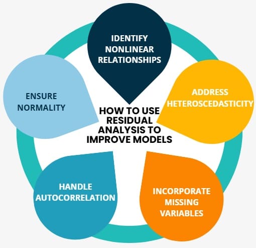
Residual analysis provides valuable information for improving regression models. Here’s how you can use the insights gained from residual plots and tests:

1. Identify Nonlinear Relationships: If residual plots show patterns like U-shapes or curved trends, it’s a sign that a nonlinear model might be needed. You can add polynomial terms or transform the variables to address this issue.
2. Address Heteroscedasticity: If you notice heteroscedasticity (non-constant variance of residuals), consider using weighted least squares regression or applying a transformation to stabilize the variance.
3. Incorporate Missing Variables: If residuals show trends that indicate missing variables, consider adding new predictors to the model.
4. Handle Autocorrelation: If residuals exhibit autocorrelation, especially in time series data, you may need to include lagged variables or use time series models like ARIMA.
5. Ensure Normality: If residuals deviate from normality, consider applying data transformations (such as log or square root transformations) or using nonparametric methods.

Final Words

Residual analysis is an essential step in regression modeling. It allows us to check if the key assumptions of the model are valid, which is crucial for ensuring that the model provides reliable and accurate predictions.

By examining the residuals through various diagnostic plots, we can identify problems such as non-linearity, heteroscedasticity, and non-normality, which could lead to incorrect conclusions or misinformed decisions. Therefore, residual analysis is not just a post-fitting check; it is an integral part of ensuring that the regression model is appropriate and robust.

Related Articles

• Residuals
• What Is Multiple Linear Regression (MLR)?
• Anderson-Darling Normality Test
• Homogeneity of Variance
• Fits