Simple linear regression is a powerful statistical tool used to model the relationship between two variables: one independent (x) and one dependent (y). Whether you’re predicting sales based on advertising spend or analyzing trends in data, this method helps you uncover patterns with ease.
Simple linear regression represents a statistical method that models the relationship between two continuous variables by fitting a linear equation to observed data. Specifically, it examines how one dependent variable (y) changes in response to changes in one independent variable (x). The method creates a straight line that best represents the relationship between these variables, allowing you to make predictions and understand patterns in your data.
In this article, we’ll break down what is linear regression, its applications, assumptions, and how to calculate it using tools like a linear regression calculator. Let’s dive in!
Table of contents
What is Simple Linear Regression?
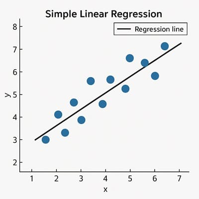
Simple linear regression is a statistical method that models the relationship between two variables by fitting a straight line, known as the regression line or line of best fit, to the data.

The goal is to predict the dependent variable (y) based on the independent variable (x) using the linear regression equation: y = mx + b, where:
- m is the slope (how much y changes for a unit change in x),
- b is the y-intercept (the value of y when x is 0).
For example, if you’re studying how study hours (x) affect exam scores (y), simple linear regression helps you predict scores based on hours spent studying. This method assumes a linear relationship, meaning the change in y is proportional to the change in x.
Furthermore, statisticians often express this equation as: y = β₀ + β₁x + ε, where β₀ is the intercept, β₁ is the slope coefficient, and ε represents the error term.
The slope indicates how much y changes for each unit increase in x, while the y-intercept shows the predicted value of y when x equals zero. Together, these parameters define your regression line and enable accurate predictions.
Public, Onsite, Virtual, and Online Six Sigma Certification Training!
- We are accredited by the IASSC.
- Live Public Training at 52 Sites.
- Live Virtual Training.
- Onsite Training (at your organization).
- Interactive Online (self-paced) training,
Why Use Simple Linear Regression?
Simple linear regression is popular because it’s:
- Easy to Understand: The y=mx+b formula is straightforward.
- Widely Applicable: Used in fields like economics, science, and machine learning.
- Efficient: Tools like regression calculators and slope intercept calculators make calculations quick.
By using a linear regression model, you can quantify relationships, make predictions, and identify trends.
Key Components of Simple Linear Regression
To master simple linear regression, you need to understand its core components:
1. The Linear Regression Equation
The linear regression equation is y = mx + b. Here’s what each term means:
- y: The dependent variable (what you’re predicting).
- x: The independent variable (what influences y).
- m: The slope, calculated as the regression coefficient, showing the change in y per unit change in x.
- b: The y-intercept, where the regression line crosses the y-axis.
You can use a y-intercept calculator or slope finder to compute these values.
2. The Regression Line
The regression line (or line of best fit) minimizes the distance between data points and the line. This is often calculated using the least squares regression line formula, which ensures the smallest possible sum of squared errors.
Also Read: What is a Regression Equation?
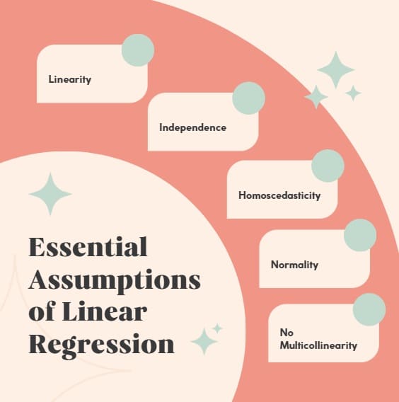
Essential Assumptions of Linear Regression

Before applying simple linear regression, you must verify several critical assumptions:
1. Linearity
The relationship between variables must be linear. Plot your data on a scatter plot to visually assess this assumption.
2. Independence
Observations should be independent of each other. Each data point shouldn’t influence others in the dataset.
3. Homoscedasticity
The variance of residuals should remain constant across all levels of the independent variable. This means the spread of data points around the regression line should be consistent.
4. Normality
The residuals should follow a normal distribution. This assumption becomes less critical with larger sample sizes due to the Central Limit Theorem.
5. No Multicollinearity
While this applies more to multiple linear regression, ensure your independent variable doesn’t have perfect correlation with other variables in extended analyses.
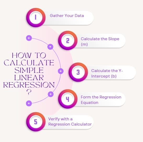
How to Calculate Simple Linear Regression?

Calculating simple linear regression involves finding the slope (m) and y-intercept (b). Here’s a step-by-step guide:
Step 1: Gather Your Data Collect paired data for your independent (x) and dependent (y) variables. For example, let’s say you have study hours and exam scores:
Hours (x)Score (y)150260375480595
Step 2: Calculate the Slope (m) The slope is calculated using the formula:
m = [n(∑xy) – (∑x)(∑y)] / [n(∑x²) – (∑x)²]
Where:
- ∑xy: Sum of the product of x and y
- ∑x: Sum of x values
- ∑y: Sum of y values
- ∑x²: Sum of squared x values
- n: Number of data points
For the above data, a slope calculator or slope finder can simplify this process.
Step 3: Calculate the Y-Intercept (b) The y-intercept is found using:
b = [∑y – m(∑x)] / n
A y-intercept calculator can compute this quickly.
Step 4: Form the Regression Equation Plug m and b into y = mx + b. For our example, if m = 10 and b = 40, the equation is y = 10x + 40. This means for every additional hour studied, the score increases by 10 points.
Step 5: Verify with a Regression Calculator Tools like a linear regression calculator or least squares regression line calculator can automate these steps. Input your data into a graph calculator or table calculator to visualize the regression line and verify your calculations.
Also Read: What is Multiple Regression Line?
Tools for Simple Linear Regression
Several online tools can streamline your calculations:
- Linear Regression Calculator: Computes the regression equation and plots the line of best fit.
- Slope and Y-Intercept Calculator: Finds m and b directly.
- Graph Calculator: Visualizes data points and the regression line.
- Linear Correlation Coefficient Calculator: Measures the strength of the linear relationship (r-value).
Popular platforms like Desmos, GeoGebra, or even Excel offer these functionalities for free.
Practical Applications of Simple Linear Regression
Simple linear regression is used across industries:
- Business: Predict sales based on marketing spend.
- Healthcare: Analyze how exercise impacts blood pressure.
- Education: Estimate test scores based on study time.
- Science: Model relationships like temperature vs. ice melt rate.
For instance, a company might use a regression equation calculator to forecast revenue based on advertising budgets, helping them allocate resources efficiently.
Simple Linear Regression vs. Multiple Linear Regression
While simple linear regression uses one independent variable, multiple linear regression involves multiple predictors. For example, predicting house prices might involve square footage (x₁), number of bedrooms (x₂), and location (x₃). The formula extends to:
y = b₀ + b₁x₁ + b₂x₂ + … + bₙxₙ
Multiple linear regression is more complex but handles multifaceted relationships. If you’re new to regression, start with simple linear regression before exploring multiple linear regression.
Common Mistakes to Avoid
To ensure accurate results, avoid these pitfalls:
- Ignoring Assumptions: Always verify linear regression assumptions like linearity and normality.
- Overfitting the Model: Don’t assume every dataset fits a linear model; consider exponential regression if the relationship is non-linear.
- Misinterpreting Correlation: A strong linear correlation coefficient doesn’t imply causation.
Visualizing Simple Linear Regression
Visualizing data helps interpret results. A graph calculator or slope graph calculator can plot your data points and the regression line. This visual aid shows how well the line fits the data and highlights outliers.
For example, plotting our study hours vs. scores data would show a clear upward trend, confirming a positive slope.
Advanced Considerations
Once you’re comfortable with simple linear regression, explore these advanced topics:
- Logistic Regression: Used for binary outcomes (e.g., pass/fail).
- Regression Coefficient Interpretation: Understand the practical significance of m and b.
- Residual Analysis: Examine residuals to check linear regression assumptions.
You can use a linearization calculator for non-linear data or an exponential regression calculator for exponential trends.
Transitioning to Multiple Linear Regression
While simple linear regression uses one predictor variable, multiple linear regression extends this concept to include several independent variables. This advanced technique follows similar principles but requires more sophisticated interpretation and assumption checking.
The transition from simple to multiple regression involves understanding how additional variables affect the model’s complexity and interpretability. However, mastering simple linear regression provides the essential foundation for these advanced techniques.
Final Words
Simple linear regression serves as a powerful tool for understanding relationships between variables and making data-driven predictions. By mastering the linear regression formula, understanding key assumptions, and properly interpreting results, you’ll be equipped to tackle a wide range of analytical challenges.
Whether you’re using a basic linear equation calculator or sophisticated statistical software, the fundamental principles remain constant. Focus on understanding the underlying concepts, checking assumptions, and interpreting results within appropriate contexts.
Frequently Asked Questions (FAQs) on Simple Linear Regression
What is the difference between simple linear regression and multiple linear regression?
Simple linear regression uses one independent variable to predict one dependent variable (y = mx + b), while multiple linear regression uses multiple independent variables to predict one dependent variable (y = b₀ + b₁x₁ + b₂x₂ + … + bₙxₙ).
How do I know if my data meets the assumptions of linear regression?
Check assumptions by creating residual plots, conducting normality tests, examining scatter plots for linearity, and testing for constant variance. Most statistical software provides diagnostic tools for assumption checking.
What does R-squared tell me about my regression model?
R-squared (coefficient of determination) indicates the percentage of variance in the dependent variable explained by the independent variable. Values range from 0 to 1, with higher values indicating better model fit.
Can I use linear regression for non-linear relationships?
Simple linear regression works best for linear relationships. For non-linear relationships, consider data transformations, polynomial regression, or non-linear regression methods.
How do I interpret the slope coefficient in practical terms?
The slope coefficient represents the average change in the dependent variable for each one-unit increase in the independent variable. For example, if studying the relationship between temperature and ice cream sales, a slope of 2 means sales increase by 2 units for each degree temperature increases.
What sample size do I need for reliable linear regression results?
While there’s no strict minimum, generally aim for at least 20-30 observations for simple linear regression. Larger samples provide more reliable estimates and better assumption checking capabilities.


