
An operating characteristic curve, commonly known as a ROC curve (Receiver Operating Characteristic), represents one of the most fundamental tools for evaluating binary classification models in machine learning. This powerful visualization technique plots the true positive rate against the false positive rate across various threshold settings, providing crucial insights into model performance.
The ROC meaning extends beyond simple accuracy metrics, offering a comprehensive view of how well your classification model distinguishes between different classes. Whether you’re working with medical diagnosis systems, fraud detection algorithms, or customer segmentation models, understanding ROC curves becomes essential for making informed decisions about model effectiveness.
Table of contents
What is an Operating Characteristic Curve?
An Operating Characteristic Curve (OC Curve) is a graphical tool used to visualize how well a sampling plan or classification model distinguishes between good and bad outcomes. In quality control, it shows the probability of accepting a batch based on its quality level or defect rate. In machine learning, it helps evaluate the performance of classification models by plotting true positive rates against false positive rates at various thresholds.
- X-axis: Quality level (e.g., percent defective) or False Positive Rate (FPR)
- Y-axis: Probability of acceptance or True Positive Rate (TPR)
The OC curve is essential for understanding and balancing the risks between producers (risk of rejecting good batches) and consumers (risk of accepting bad batches).

Public, Onsite, Virtual, and Online Six Sigma Certification Training!
- We are accredited by the IASSC.
- Live Public Training at 52 Sites.
- Live Virtual Training.
- Onsite Training (at your organization).
- Interactive Online (self-paced) training,
Operating Characteristic Curve Curve in Quality Control
In manufacturing and quality assurance, the OC curve is a staple for acceptance sampling. It helps managers and engineers decide whether to accept or reject production lots based on sample inspections.
- Producer’s Risk (α): Probability of rejecting a good lot (at Acceptable Quality Level, AQL)
- Consumer’s Risk (β): Probability of accepting a bad lot (at Rejectable Quality Level, RQL)
An ideal OC curve drops sharply from a high probability of acceptance to a low probability near the AQL, indicating a precise sampling plan.
What Does ROC Stand For?
ROC stands for Receiver Operating Characteristic, a term originally developed during World War II for analyzing radar signals. Today, this concept has evolved into a cornerstone of machine learning evaluation, particularly for binary classification tasks.
The ROC definition encompasses both the curve itself and the underlying methodology for assessing classification performance. When data scientists ask “what is ROC,” they’re referring to this comprehensive evaluation framework that considers both sensitivity and specificity simultaneously.
Key Components of ROC Analysis
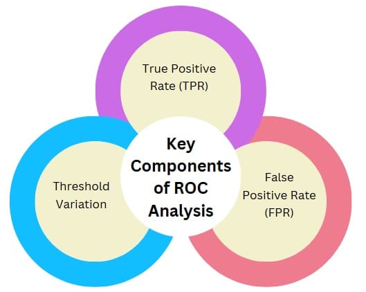
ROC analysis involves several critical components that work together to provide meaningful insights:
True Positive Rate (TPR): Also known as sensitivity or recall, TPR measures the proportion of actual positive cases correctly identified by the model. The purpose of a TPR graph is to visualize how effectively your model captures positive instances across different thresholds.
False Positive Rate (FPR): This metric represents the proportion of actual negative cases incorrectly classified as positive, directly impacting the specificity of your model.
Threshold Variation: ROC curves demonstrate model performance across multiple decision thresholds, revealing how threshold selection affects classification outcomes.
Also Read: What is Failure Rate?
What is AUC?
The Area Under the Curve (AUC) provides a single numerical summary of ROC curve performance. AUC meaning encompasses the probability that your model will rank a randomly chosen positive instance higher than a randomly chosen negative instance.
AUC scores range from 0 to 1, where:
- AUC = 1.0 indicates perfect classification
- AUC = 0.5 suggests random performance
- AUC < 0.5 implies worse-than-random performance
Understanding AUC-ROC Relationships
The relationship between AUC and ROC curves creates a powerful evaluation metric. AUC ROC scores help practitioners compare different models objectively, making it easier to select the best-performing algorithm for specific applications.
AUROC (Area Under the ROC Curve) serves as another common abbreviation for this metric, particularly in academic and research contexts. The AUC metric provides valuable insights regardless of class distribution, making it especially useful for imbalanced datasets.
How to Calculate and Interpret ROC Curves?
ROC Formula and Calculation Methods
Calculating AUC involves several approaches, from geometric approximations to trapezoidal integration. The fundamental AUC formula uses the trapezoidal rule to estimate the area under the ROC curve:
AUC = Σ(TPR_i + TPR_i+1) × (FPR_i+1 – FPR_i) × 0.5
However, most machine learning libraries provide built-in functions for AUC calculation, simplifying this process for practitioners.
Practical Steps for ROC Analysis
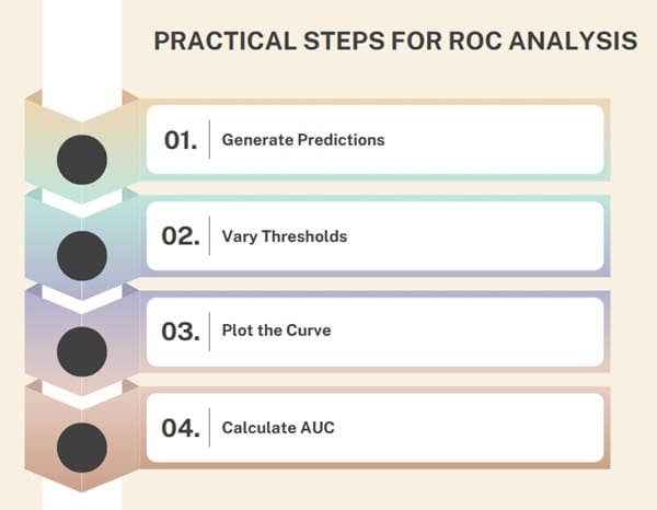
Creating effective ROC plots involves several systematic steps:
- Generate Predictions: Apply your trained model to generate probability scores for test data
- Vary Thresholds: Calculate TPR and FPR values across different decision thresholds
- Plot the Curve: Create the ROC curve by plotting TPR against FPR
- Calculate AUC: Compute the area under the ROC curve for quantitative assessment
Interpreting ROC Curve Shapes
Different ROC curve shapes reveal important information about model behavior:
Steep Initial Rise: Indicates excellent performance at low false positive rates Diagonal Line: Suggests random classification performance Concave Shape: May indicate potential issues with model calibration.
AUC in Machine Learning Applications
Classification Performance Evaluation
AUC in machine learning serves multiple purposes beyond simple model comparison. The metric helps practitioners understand trade-offs between sensitivity and specificity, crucial for applications where false positives and false negatives carry different costs.
Classification in machine learning benefits significantly from ROC analysis, particularly when dealing with:
- Medical diagnosis systems
- Fraud detection algorithms
- Spam filtering applications
- Risk assessment models
Advanced AUC Interpretations
AUC machine learning applications extend beyond binary classification through techniques like:
- Multi-class ROC analysis
- Micro and macro-averaged AUC scores
- Time-series ROC evaluation
- Cross-validation AUC assessment
ROC Analysis in Different Domains
Medical Applications
In healthcare, ROC medical abbreviation usage remains widespread for diagnostic test evaluation. Medical professionals rely on ROC analysis to:
- Assess diagnostic accuracy
- Compare different testing procedures
- Optimize decision thresholds for patient care
- Evaluate screening program effectiveness
AI and Machine Learning Integration
ROC AI applications continue expanding as artificial intelligence systems become more sophisticated. Modern ROC training methodologies incorporate:
- Deep learning model evaluation
- Ensemble method assessment
- Automated hyperparameter optimization
- Real-time performance monitoring
Advanced ROC Concepts and Variations
Beyond Basic ROC Analysis
While standard ROC curves provide valuable insights, advanced practitioners often utilize specialized variations:
Precision-Recall Curves:
Particularly useful for highly imbalanced datasets where ROC curves might be overly optimistic
Cost-Sensitive ROC:
Incorporates different costs for false positives and false negatives
Confidence Intervals:
Provides statistical significance testing for AUC comparisons
Multi-Class Extensions
Extending ROC-AUC analysis to multi-class problems involves:
- One-vs-Rest (OvR) ROC curves
- One-vs-One (OvO) comparisons
- Macro and micro-averaged metrics
- Volume Under Surface (VUS) calculations
Also Read: What is Acceptable Quality Level?
Best Practices for ROC Implementation
Data Preparation Considerations
Effective ROC analysis requires careful attention to:
- Data Quality: Ensuring clean, representative datasets
- Sample Size: Maintaining sufficient data for reliable estimates
- Class Balance: Understanding how imbalanced data affects interpretation
- Cross-Validation: Implementing robust validation strategies
Common Pitfalls and Solutions
Practitioners should avoid these frequent mistakes:
- Overfitting Concerns: Using the same data for training and ROC evaluation
- Threshold Selection: Choosing thresholds based solely on ROC appearance
- Metric Misinterpretation: Misunderstanding AUC limitations in specific contexts
Tools and Technologies for ROC Analysis
Programming Libraries and Frameworks
Modern ROC curve implementation benefits from numerous tools:
- Python: scikit-learn, matplotlib, seaborn
- R: pROC, ROCR, ggplot2
- Commercial Software: SPSS, SAS, MATLAB
Visualization Best Practices
Creating effective AUROC curves requires attention to:
- Clear axis labeling and scaling
- Appropriate color schemes and line styles
- Confidence interval visualization
- Multiple model comparisons
Frequently Asked Questions (FAQ) on Operating Characteristic Curve
What does ROC stand for in machine learning?
ROC stands for Receiver Operating Characteristic, a method for evaluating binary classification model performance by plotting true positive rate against false positive rate.
How do you calculate AUC from an ROC curve?
AUC is calculated as the area under the ROC curve, typically using trapezoidal integration or built-in machine learning library functions that compute this automatically.
What is a good AUC score?
AUC scores range from 0 to 1, where 0.8-0.9 is considered good, 0.9-1.0 is excellent, and 0.5 represents random performance equivalent to chance.
When should you use ROC curves instead of other metrics?
ROC curves work best for balanced datasets and when you need to understand trade-offs between sensitivity and specificity across different thresholds.
What is the difference between AUC and AUROC?
AUC and AUROC refer to the same metric – Area Under the ROC Curve. AUROC is simply a more explicit abbreviation that specifies the ROC curve context.
Can ROC curves be used for multi-class classification?
Yes, through one-vs-rest or one-vs-one approaches, though precision-recall curves often provide better insights for multi-class problems.