Coefficient of Determination (R²): What It Really Tells You

The coefficient of determination, written R² and read “R-squared,” is the proportion of variation in an output (Y) that a regression model explains using its input variable(s), expressed as a value between 0 and 1, or 0% to 100%.

An R² of 0.75 means the model explains 75% of the variation in the outcome, leaving 25% unexplained by anything in the model. What almost every basic explanation leaves out is the more important, more dangerous fact: a high R² does not automatically mean a good model, and a low R² does not automatically mean a bad one.

This guide covers the real formula, why R² always increases when you add more variables regardless of whether they help, the adjusted and predicted R² fixes for that problem, and the specific mistakes that lead Six Sigma teams to trust a regression model they shouldn’t.

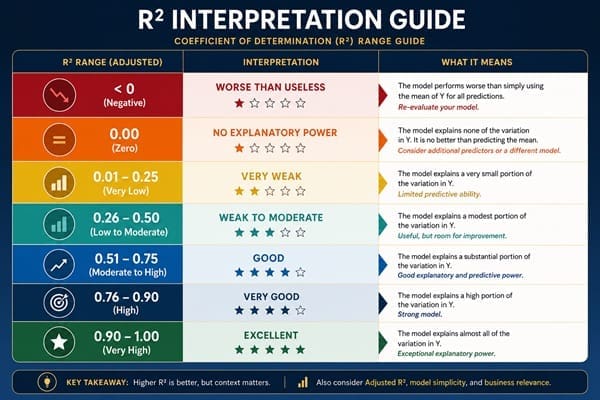
R² Range	What It Suggests	Important Caveat
0.90 to 1.00	Model explains most of the variation	Check for overfitting, especially with many predictors and a small sample
0.70 to 0.89	Strong explanatory power	Confirm with residual plots that the model is genuinely a good fit
0.50 to 0.69	Moderate explanatory power	Often acceptable in fields with high natural variability
Below 0.50	Weak explanatory power by itself	Not automatically a bad model; some outcomes are inherently harder to predict
Negative (adjusted R²)	Model performs worse than simply using the mean	A clear signal the model or its variables need to be reconsidered

Key Takeaways

• R² measures explained variation, not accuracy or causation. A model can have a high R² and still make poor predictions, or have a low R² and still be a legitimately useful model, depending on the field and the data.
• R² will always increase, or at worst stay the same, every time you add another variable to a model, even a completely irrelevant one. This is a mathematical property of the formula, not a sign of a genuinely better model.
• Adjusted R² corrects for that problem by penalizing the addition of variables that don’t meaningfully improve the model, making it the more honest metric when comparing models with different numbers of predictors.
• Predicted R² catches overfitting that adjusted R² can miss, by testing how well the model predicts data points it wasn’t built on, using a systematic leave-one-out process.
• There is no universal “good” R² value. What counts as strong depends heavily on the field: physical, controlled manufacturing processes often produce high R² values, while processes involving human behavior or highly variable inputs often produce legitimately useful models with much lower R².

What Is the Coefficient of Determination?

The coefficient of determination (R²) is a statistic that quantifies how much of the variation in a dependent variable (Y) is explained by the independent variable or variables (X) in a regression model. It answers a specific, practical question: if I use this model to predict Y, how much of the actual spread in Y does the model account for, versus how much is left over as unexplained noise?

The formula behind R² compares two quantities: the sum of squared differences between the actual data points and the model’s predicted values (the unexplained variation), against the sum of squared differences between the actual data points and the simple average of Y (the total variation).

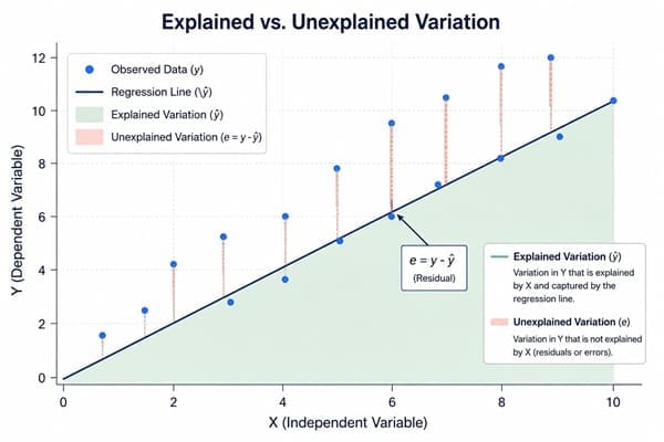
R² is calculated as 1 minus the ratio of those two quantities. When a model’s predictions land exactly on every actual data point, unexplained variation is zero and R² equals 1. When a model explains nothing beyond simply guessing the average every time, R² equals 0.

For simple linear regression with one predictor, R² is mathematically identical to the square of the Pearson correlation coefficient (r) between the predictor and the outcome. This is a useful shortcut to remember, but it also means R² inherits correlation’s core limitation: it measures the strength of a relationship, not whether that relationship is causal.

The Trap Almost Every Basic Explanation Misses: R² Always Goes Up

This is the single most important practical fact about R², and it is the reason a Six Sigma practitioner should never evaluate a regression model on R² alone.

According to statistical guidance on regression model evaluation, adding more independent variables to a model will always increase R², or at worst leave it unchanged, even when those additional variables have no real predictive relationship with the outcome.

This happens because of how the underlying math works: an extra variable can only ever help the model fit the specific dataset used to build it better, never worse, purely by chance if nothing else.

The practical danger is obvious once you see it: a team chasing a higher R² by throwing more input variables into a regression model isn’t necessarily building a better model. They may just be building a more complicated one that fits their specific sample of data suspiciously well, while becoming worse at predicting anything new.

Also Read: Correlation Coefficient

The Fix: Adjusted R² and Predicted R²

Two related statistics exist specifically to correct the problem above, and understanding both is what separates a rigorous regression analysis from a superficial one.

Adjusted R² penalizes a model for adding variables that don’t meaningfully improve its explanatory power. Unlike standard R², adjusted R² can actually decrease when an irrelevant predictor is added, which makes it the correct metric to use whenever comparing two models that contain different numbers of input variables. A model with a lower standard R² but a higher adjusted R² than a competing model is often the more honest, more generalizable choice.

Predicted R² goes a step further and directly tests for overfitting. According to guidance on regression diagnostics, predicted R² is calculated by systematically removing one data point at a time, refitting the model without it, and evaluating how well the resulting model predicts the missing point, repeating this process across the entire dataset.

A model that fits its own training data extremely well but produces a much lower predicted R² is a model that has been overfit: it has essentially memorized its own sample rather than learned a genuinely predictive relationship, and it should not be trusted to perform well on new process data going forward.

A telling warning sign: adjusted R² can turn negative. A negative adjusted R² means the model’s predictors, taken together, explain the outcome worse than simply using the average of Y every single time, a strong signal that the current model or variable selection needs to be reconsidered entirely rather than fine-tuned.

Why “Higher Is Always Better” Is the Wrong Mindset

Six Sigma practitioners coming from a manufacturing background sometimes assume a strong regression model should always produce a high R², because physical, tightly controlled processes often do. But that assumption breaks down the moment the outcome being modeled has more inherent, irreducible variability.

According to regression interpretation guidance, some fields of study have an inherently greater amount of unexplainable variation, and studies trying to explain human behavior, for example, commonly produce R² values below 50 percent while still representing legitimately useful models.

A regression model predicting call center agent satisfaction scores from measurable factors will almost never reach the R² a model predicting machine cycle time from feed rate and pressure can reach, not because the analysis is worse, but because human behavior carries more unmodeled variability than a physical process does.

The reverse trap is just as real: a suspiciously high R², especially one near 0.95 or above with several predictors and a modest sample size, deserves scrutiny rather than celebration. It is often a sign of overfitting rather than genuine predictive insight.

Where the Coefficient of Determination Fits Inside DMAIC

R² earns its place specifically in the Analyze and Improve phases, wherever a Six Sigma team is building a regression model to understand or predict a process outcome.

In the Analyze phase, R² helps a team evaluate whether a suspected input variable, or combination of variables, genuinely explains meaningful variation in a defect rate, cycle time, or other outcome, before committing further investigation resources to that variable. In the Improve phase, particularly during Design of Experiments work, R² and adjusted R² help confirm that a fitted response surface model (the kind of model behind a contour plot) is trustworthy enough to base process optimization recommendations on.

In neither phase should R² be the only number reported; residual plots, adjusted and predicted R², and a basic sanity check against domain knowledge should always accompany it.

Real Examples of Coefficient of Determination in Practice

Manufacturing: Cycle Time Prediction

A team builds a regression model predicting machine cycle time from feed rate and tool wear, achieving an R² of 0.91. Because the process is physical and tightly controlled, this high R² is plausible, though the team still checks adjusted R² to confirm neither variable is redundant.

Healthcare: Predicting Patient Length of Stay

A hospital builds a model predicting patient length of stay from admission diagnosis, age, and comorbidity count, achieving an R² of only 0.38. Rather than discarding the model as weak, the team recognizes that patient outcomes carry substantial inherent variability, and a model explaining over a third of that variation is still operationally useful for staffing forecasts.

Retail: Overfitting a Sales Forecast Model

An analyst adds twelve input variables to a sales forecasting model and watches standard R² climb to 0.97. Checking predicted R², the team discovers it drops to 0.52, revealing the model has been overfit to historical data and would likely perform poorly forecasting a new sales period.

Also Read: Paper Clearance Time Improvement

Common Mistakes When Using the Coefficient of Determination

• Treating a high R² as proof the model is correct. R² measures explained variation, not whether the model’s assumptions, like linearity, are actually valid for the data.
• Adding variables purely to chase a higher R². Since R² mechanically increases with more variables regardless of relevance, this practice produces bloated, overfit models rather than better ones.
• Comparing standard R² across models with different numbers of predictors. This comparison is invalid; adjusted R² is the correct metric for that specific comparison.
• Never checking predicted R² or residual plots. A model that looks excellent by R² alone can still be a poor predictor of new data, and only these additional checks reveal that.
• Applying a single universal “good R²” threshold across every field. What counts as a strong R² in a controlled manufacturing process is a very different bar than what counts as strong in a process involving human behavior.

Frequently Asked Questions (FAQs) on Coefficient of Determination

What is a good R-squared value?

There is no universal answer. Physical, tightly controlled processes often produce R² values above 0.80, while processes involving significant human behavior or uncontrolled variability can produce legitimately useful models with R² values well below 0.50.

What is the difference between R-squared and adjusted R-squared?

R-squared always increases, or stays the same, when a new variable is added to a model, regardless of whether that variable is meaningful. Adjusted R-squared penalizes irrelevant variables and can decrease when they’re added, making it the correct metric for comparing models with different numbers of predictors.

Can R-squared be negative?

Standard R² cannot go below 0, but adjusted R² can turn negative. A negative adjusted R² means the model performs worse than simply predicting the average outcome every time, a clear signal to reconsider the model.

Does a high R-squared mean the model is good?

Not necessarily. A high R² can result from overfitting, especially with many predictors and a small sample size. Predicted R² and residual plots are needed to confirm a model genuinely generalizes beyond its own training data.

How is R-squared related to the correlation coefficient?

For simple linear regression with one predictor, R² equals the square of the Pearson correlation coefficient (r) between the predictor and the outcome. This relationship does not hold the same way once multiple predictors are involved.

Final Words

The coefficient of determination answers a narrower question than most people assume: how much variation does this specific model explain, not whether the model is correct, causal, or generalizable. Understanding adjusted and predicted R², and recognizing that “higher is always better” is often the wrong instinct, is what separates a Six Sigma practitioner who trusts a regression model blindly from one who knows how to stress-test it first.

Six Sigma Development Solutions Inc. teaches regression analysis, R² interpretation, and the full DOE statistical toolkit through onsite, live virtual, public, and online formats. Our Black Belt certification course works through real Minitab regression output and overfitting diagnostics, not just theory. View our upcoming Black Belt training schedule and get $500 off your next class.

Lean Six Sigma Green Belt Training Brochure

Related Articles

• What Is Multiple Linear Regression (MLR)?
• Fits
• Correlation Coefficient
• Process Control
• Simple Linear Regression: A Complete Guide for Six Sigma Practitioners