
Moment statistics refers to the use of moments to describe the shape and key features of a probability distribution. In the field of statistics, a moment is essentially a specific quantitative measure of the shape of a set of points. These measures help to summarize the characteristics of a random variable’s distribution.
The concept of a moment comes from physics, where it is used to describe the distribution of mass or force.
In moment statistics, instead of mass, we are looking at the distribution of probability or data points around a central value.
Moment statistics are crucial tools in descriptive statistics. They are used extensively across various fields, including finance, engineering, and data science, to gain a deep understanding of data distributions.
Table of contents
Definition of Moment
The moment of a random variable X is defined as the expected value of a power of that random variable. We can write this definition mathematically.
The r-th moment of a random variable X about a point c is the Expected Value of the quantity (X−c) raised to the power of r.
In simple terms, the formula is:
The r-th Moment = The Average Value of (X−c)^r
Here, E stands for the Expected Value, which is the long-run average. The value r is the order of the moment. We commonly use moments calculated about two key points: the origin (c=0) and the mean (μ).

Public, Onsite, Virtual, and Online Six Sigma Certification Training!
- We are accredited by the IASSC.
- Live Public Training at 52 Sites.
- Live Virtual Training.
- Onsite Training (at your organization).
- Interactive Online (self-paced) training,
Types of Moments in Moment Statistics
In moment statistics, there are two primary types of moments that statisticians use: Raw Moments and Central Moments. Each type provides different, yet related, information about the data’s distribution.
1. Raw Moments (Moments about the Origin)
Raw moments, also called moments about the origin, are calculated by setting the point c=0 in the general formula.
The r-th raw moment is calculated as:
The r-th Raw Moment = The Average Value of (X)^r
Raw moments help to locate the center of the distribution and describe its spread.
First Raw Moment: The first raw moment is the Expected Value of X, which is the mean (μ) of the distribution. The mean is the center of mass for the distribution.
Second Raw Moment: The second raw moment is the Expected Value of X^2. This value is used to calculate the variance.
2. Central Moments (Moments about the Mean)
Central moments are calculated by setting the point c equal to the mean (μ) of the random variable X.
The r-th central moment (μ_r) is calculated as:
The r-th Central Moment = The Average Value of (X−μ)^r
Central moments are more important for describing the shape of the distribution, as they are independent of the distribution’s location.
First Central Moment: The first central moment is always zero. This is the average value of the distance of all data points from the mean.
Second Central Moment: The second central moment is the variance (σ^2). Variance is the average squared distance from the mean.
Third Central Moment: The third central moment is used to measure the skewness of the distribution.
Fourth Central Moment: The fourth central moment is used to measure the kurtosis of the distribution.
The Four Moments: Detailed Explanation
In practice, when discussing moment statistics, statisticians usually focus on the first four central moments. These four moments are the fundamental tools for describing a distribution’s shape completely.
| Order (r) | Central Moment Symbol | Name/Concept | What it Measures |
| 1st | μ_1 (is always 0) | Zero | Location of the mean (Always zero) |
| 2nd | μ_2 or σ^2 | Variance | Spread or Dispersion |
| 3rd | μ_3 | Skewness | Symmetry of the distribution |
| 4th | μ_4 | Kurtosis | Tail Shape and Peakedness |
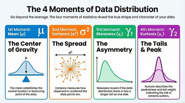
1. The First Moment: Mean (μ)
The first moment (specifically, the first raw moment) defines the location of the distribution. The symbol μ (pronounced ‘mew’) is used for the mean.
Mean is the arithmetic average of all the values in the dataset.
Mean is often the first statistic calculated for any dataset because it anchors the distribution.
In moment statistics, the mean acts as the balancing point or the center of gravity for the data.
2. The Second Moment: Variance and Standard Deviation
The second central moment (μ_2) is the variance (σ^2). The symbol σ (pronounced ‘sigma’) represents the standard deviation. This moment measures the dispersion or spread of the data points.
Variance quantifies how far the numbers in a set are spread out from their mean value. A high variance suggests the data is widely scattered.
Standard Deviation (σ) is the square root of the variance. It is a more interpretable measure because it is in the same units as the original data.
Why is understanding the spread so important? Knowing the spread tells you about the risk in finance or the consistency in a manufacturing process.
3. The Third Moment: Skewness
The third central moment (μ_3) is the basis for measuring skewness. Skewness is a measure of the asymmetry of the distribution.
A distribution can be:
Symmetrical: The right side is a mirror image of the left side. The skewness value is approximately zero. (e.g., a perfect normal distribution).
Positively Skewed (Right-Skewed): The tail extends toward the right (positive) side. The skewness value is positive. This often occurs when there are a few very large values pulling the mean up. (For example, income distribution).
Negatively Skewed (Left-Skewed): The tail extends toward the left (negative) side. The skewness value is negative.
To get a standardized measure of skewness (γ_1), we divide the third central moment by the standard deviation cubed.
In simple terms, the formula for standardized skewness (γ_1) is:
Skewness (γ_1) = Third Central Moment / (Standard Deviation)^3
Skewness is a vital tool for understanding the structure of a dataset. Does your data have a long tail of extreme values? Moment statistics with the third moment can reveal this structure.
4. The Fourth Moment: Kurtosis
The fourth central moment (μ_4) is the basis for measuring kurtosis. Kurtosis describes the shape of the tails and the peakedness of the distribution relative to a normal distribution.
To get a standardized measure of excess kurtosis (γ_2), we divide the fourth central moment by the variance squared, and then subtract three.
In simple terms, the formula for excess kurtosis (γ_2) is:
Excess Kurtosis (γ_2) = Fourth Central Moment / (Variance)^2 − 3
The subtraction of three ensures that a standard normal distribution has a kurtosis of zero.
Mesokurtic: The excess kurtosis is approximately zero. This is the shape of a normal distribution.
Leptokurtic: The excess kurtosis is positive (>0). The distribution has heavier, fatter tails and a sharper peak than the normal distribution. This means more of the variance comes from extreme values.
Platykurtic: The excess kurtosis is negative (<0). The distribution has lighter, thinner tails and a flatter peak than the normal distribution.
Kurtosis is especially important in finance for assessing “tail risk”—the likelihood of extreme positive or negative outcomes. Moment statistics give you the power to find these key differences in risk.
Comparison of Raw Moments and Central Moments
When studying moment statistics, it is essential to know the key differences between the two main types of moments. This comparison helps you choose the right tool for analyzing a distribution.
| Basis for Comparison | Raw Moments (μ’_r) | Central Moments (μ_r) |
| Meaning | Moments calculated about the origin (c=0). | Moments calculated about the mean (μ). |
| Formula Concept | Average Value of (X)^r. | Average Value of (X−μ)^r. |
| Purpose | Primarily used to find the mean and simplify the calculation of central moments. | Primarily used to describe the shape of the distribution (variance, skewness, kurtosis). |
| Location Dependent | Yes. A change in the location (mean) of the data will change all raw moments. | No. They are independent of the location (mean) of the data. |
| First Moment | The mean of the distribution (μ). | Always zero. |
| Second Moment | E[X^2]. Used to calculate variance. | The variance (σ^2). |
Raw moments are a starting point. Central moments give the real information about a distribution’s characteristics. Therefore, the core of moment statistics lies in using central moments.
Advantages of Using Moment Statistics
Moment statistics provide a concise and powerful way to summarize large amounts of data. Using the four central moments offers distinct advantages in data analysis.
Complete Description: The four central moments (mean, variance, skewness, kurtosis) provide a very rich, four-number summary of a distribution’s key features.
Simple Interpretation: Each moment has a clear, interpretable meaning (center, spread, symmetry, peakedness) that is easy for analysts to communicate.
Consistency: The mathematical foundation of moment statistics ensures that these measures are consistent and reliable across different datasets and statistical models.
Foundation for Models: Moments are used to estimate the parameters of many probability distributions (e.g., normal, gamma, or beta distribution). The method of moments is a technique for finding these estimates.
The Moment-Generating Function
In advanced moment statistics, the Moment-Generating Function (MGF) is a truly elegant concept. It is a single function that can generate all the moments of a distribution.
The MGF of a random variable X, denoted M_X(t), is the Expected Value of e^(tX).
Generating Moments: The great power of the MGF is that the r-th raw moment can be found by taking the r-th derivative of the MGF and then setting the variable t to zero.
Uniqueness: A key property is that if two distributions have the same MGF, they must be the same distribution. This makes the MGF a powerful tool for proving distribution equivalences in moment statistics.
Final Words
Moment statistics are not just abstract mathematical concepts. They are the language of data analysis. Every time a financial analyst talks about volatility (variance/second moment) or a risk manager discusses tail events (kurtosis/fourth moment), they are using this foundational area of statistics.
Understanding the four moments is the first step in moving beyond simple averages to truly analyze the hidden shapes and risks within your data. Furthermore, using these moments helps you select the correct statistical model for prediction. Moment statistics enable you to see the complete picture of a dataset.
Key Takeaways
- Moment statistics use quantitative measures to describe the shape of a probability distribution.
- The two main types are Raw Moments (about the origin) and Central Moments (about the mean).
- The four most important central moments are the mean (1st Raw), variance (2nd), skewness (3rd), and kurtosis (4th).
- Variance describes data spread, skewness describes symmetry, and kurtosis describes peakedness and tail weight.
- The Moment-Generating Function can generate all moments of a distribution through differentiation.
Frequently Asked Questions (FAQs)
1. What is the difference between raw moments and central moments?
Raw moments are calculated from the origin (zero point), while central moments are calculated from the mean of the distribution. Raw moments help locate the distribution’s center, whereas central moments describe the distribution’s shape independently of its location. Central moments are generally more useful for understanding distribution characteristics like spread, symmetry, and tail behavior.
2. Why is the first central moment always zero?
The first central moment measures the average distance of all data points from the mean. Since the mean is the balancing point of the distribution, the positive and negative deviations from the mean cancel each other out, always resulting in zero.
3. How do I interpret a positive skewness value?
A positive skewness indicates that the distribution has a longer tail extending toward the right (higher values). This means there are a few unusually large values in your dataset. Common examples include income distributions, where most people earn moderate amounts but a few earn extremely high incomes.
4. What does high kurtosis tell me about my data?
High (positive) excess kurtosis indicates that your distribution has heavier tails and a sharper peak compared to a normal distribution. This means your data has more extreme values (outliers) than would be expected in a normal distribution. In finance, this signals higher tail risk or the possibility of extreme events.
5. Can I use moment statistics for non-numeric data?
No, moment statistics require numeric data because they involve mathematical operations like taking powers and calculating expected values. For categorical or qualitative data, you would need different statistical measures like frequencies, modes, or chi-square tests.