
Imagine your team runs a hypothesis test and the data says: the improvement worked. Defect rates are down. The result is statistically significant. Everyone is ready to celebrate.
But there is a question worth asking before you do: what if the data is wrong?
Not because of a calculation error. Not because of bad data collection. Simply because of the inherent uncertainty in any statistical test — the unavoidable possibility that a significant-looking result happened by chance.
That probability has a name. It is called alpha risk.
Understanding alpha risk is not just an exam topic for Green Belt and Black Belt candidates. It is a practical skill that protects your team from making expensive decisions based on statistical noise.
Table of contents
What Is Alpha Risk?
Alpha risk (α) is the probability of incorrectly rejecting a null hypothesis that is actually true.
In plain terms: it is the risk of concluding that something changed, or that a difference exists, when in reality nothing changed at all. The observed result was a product of random sampling variation, not a genuine effect.
This type of error has several names in statistics and Six Sigma:
- Alpha risk (the most common term in Six Sigma)
- Type I error
- False positive
- Producer’s risk (in the context of acceptance sampling)
The standard alpha level used in most Six Sigma and business applications is 0.05, meaning there is a 5% chance of making this error. At this level, if you ran the same hypothesis test 100 times on data where no real difference exists, you would expect to see a statistically significant result approximately five times purely by chance.

Public, Onsite, Virtual, and Online Six Sigma Certification Training!
- We are accredited by the IASSC.
- Live Public Training at 52 Sites.
- Live Virtual Training.
- Onsite Training (at your organization).
- Interactive Online (self-paced) training,
The Null Hypothesis and What Rejection Means
To understand alpha risk fully, you need to understand what you are testing against.
Every hypothesis test starts with a null hypothesis (H₀). The null hypothesis represents the default position: no difference exists, no change has occurred, the process has not improved. It is the claim you are trying to disprove with your data.
The alternative hypothesis (Hₐ) is what you want to show: a real difference exists, the improvement worked, the two groups are not the same.
When your test produces a p-value below the alpha threshold, you reject the null hypothesis in favor of the alternative. You are saying: the data is unlikely enough under the null hypothesis that we conclude the null is probably false.
Alpha risk is the probability that this conclusion is wrong — that you rejected a true null hypothesis.
Also Read: Biggest Risks Six Sigma Faces Without a Governing Body
Alpha Risk and the P-Value: How They Connect
The p-value and the alpha level work together as a decision rule.
Alpha (α) is the threshold you set before running the test. It represents the maximum probability of a Type I error you are willing to accept. The most common value is 0.05 (5%).
The p-value is calculated from your sample data after the test runs. It represents the probability of observing a result as extreme as yours — or more extreme — if the null hypothesis were actually true.
The decision rule is straightforward:
- If the p-value ≤ alpha: reject the null hypothesis. The result is statistically significant.
- If the p-value > alpha: fail to reject the null hypothesis. The evidence is not strong enough.
When the p-value is 0.03 and alpha is 0.05, you reject the null. There is a 3% chance of seeing this result by chance alone — below your acceptable risk threshold. When the p-value is 0.08 and alpha is 0.05, you do not reject the null. The result does not clear the bar.
One important point: setting alpha at 0.05 does not mean every significant result has a 5% chance of being wrong. It means that, across many tests conducted correctly under a true null hypothesis, 5% would produce false positives. The alpha is a long-run error rate, not a verdict on any single result.
Alpha Risk as Producer’s Risk
In acceptance sampling — a quality control method used to decide whether to accept or reject a batch of incoming or outgoing product — alpha risk carries a specific operational meaning called Producer’s Risk.
Here is the scenario: a manufacturer produces a batch of parts. The batch is actually good — it meets specification. But a random sample is drawn, and due to sampling variation, the sample appears to contain more defects than the acceptable quality level. The batch is rejected.
The producer loses revenue on good product. That loss is the cost of alpha risk.
The name “Producer’s Risk” reflects who bears the consequence: the manufacturer who made good parts but saw them rejected. It is a false positive — a good batch called bad.
This framing helps make alpha risk concrete for quality professionals. It is not just a statistical abstraction. Every time you set an alpha level, you are deciding how much false-positive error you are willing to tolerate.
Also Read: Enterprise Risk Management (ERM)
Alpha Risk vs Beta Risk: Two Sides of the Same Problem
Alpha risk does not exist in isolation. Every hypothesis test involves two possible errors, and they pull in opposite directions.
Alpha risk (Type I error): Rejecting a true null hypothesis. Concluding a difference exists when it does not. A false positive. The cost is typically wasted resources — implementing a change, triggering an investigation, or rejecting good product when none of that was warranted.
Beta risk (Type II error): Failing to reject a false null hypothesis. Concluding no difference exists when one does. A false negative. The cost is a missed improvement — continuing a defective process, shipping bad product, or failing to detect a real shift in performance.
The two risks are mathematically linked. For a fixed sample size and process variation, reducing alpha (tightening your standard for significance) increases beta (making it harder to detect a real difference). You cannot reduce both simultaneously without increasing your sample size.
This trade-off has a name: statistical power. Power is defined as 1 − beta. It is the probability of correctly detecting a real difference when one exists. Higher power means lower beta risk.
The practical implication is that before collecting data, a Six Sigma practitioner should decide:
- What alpha level is acceptable for this test?
- What beta level (or power level) is acceptable?
- What is the minimum difference the team needs to detect?
These three inputs, combined with an estimate of process variation, determine the required sample size. Skipping this planning step is one of the most common and costly mistakes in Six Sigma projects — the team runs a test, gets a non-significant result, and then wonders whether the improvement was real but the test lacked the power to detect it.
How to Set Your Alpha Level
The default alpha of 0.05 is a convention, not a law. The right alpha level depends on the consequences of being wrong.
Use a lower alpha (0.01 or even 0.001) when the cost of a false positive is high. If incorrectly concluding that a medical treatment works could lead to patient harm, or if wrongly approving a manufacturing change could cause a costly recall, a stricter threshold reduces the risk of acting on a false signal.
Use the standard alpha (0.05) for most business and process improvement decisions. It represents a reasonable balance between the risk of false positives and the ability to detect real effects.
Use a higher alpha (0.10) in early-stage, exploratory analysis where you are screening for potential factors to investigate further. Missing a real lead (high beta risk) is more costly here than following up on a false one.
Whatever level you choose, set it before you run the test, not after you see the p-value. Choosing an alpha based on the result is a form of data manipulation that invalidates the statistical inference.
Also Read: Common Barriers and Risks to a Successful Six Sigma Change Project
Alpha Risk in the DMAIC Framework
Alpha risk is most visible in the Analyze and Improve phases of DMAIC, where hypothesis testing is used to confirm root causes and validate solutions. But its implications extend across the full project.
Measure phase: When establishing a baseline, confidence intervals reflect alpha risk. A 95% confidence interval corresponds to a 5% alpha — the same threshold used in hypothesis testing.
Analyze phase: Every hypothesis test run to validate a suspected root cause carries an alpha risk. Run enough tests, and the cumulative probability of at least one false positive rises significantly — a problem called multiple comparisons, or “alpha inflation.” Experienced practitioners account for this when interpreting results from screening studies.
Improve phase: When testing whether a proposed solution delivers a statistically significant improvement, alpha risk determines whether the team can confidently claim the change worked.
Control phase: When monitoring processes with control charts, the control limits are set to balance the risk of false alarms (analogous to alpha risk) against the risk of missing real shifts. Tighter limits catch shifts faster but generate more false alerts.
A Real-World Example
A Six Sigma team is testing whether a new supplier’s component reduces defect rates compared to the current supplier. They run a two-sample t-test with an alpha of 0.05.
The test returns a p-value of 0.04. They reject the null hypothesis and conclude the new supplier produces fewer defects. Based on this, the company switches suppliers.
But there is a 5% chance — the alpha they accepted — that this result occurred by chance. The null hypothesis was actually true: both suppliers produce at the same defect rate. The team made a Type I error.
The consequence: switching suppliers disrupted the supply chain, incurred transition costs, and ultimately produced no improvement. A classic false positive with a measurable business cost.
Had the team used a lower alpha of 0.01, the p-value of 0.04 would not have cleared the threshold. They would have collected more data before making the switch.
This is not a reason to set alpha at zero — that is impossible. It is a reason to set alpha deliberately, with an honest assessment of the cost of being wrong.
The Alpha Risk and Beta Risk Trade-Off: A Decision Framework
Before running any hypothesis test in a Six Sigma project, work through this sequence:
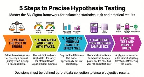
Step 1 — Define the consequences of each error type. What happens if you reject a true null (alpha error)? What happens if you fail to reject a false null (beta error)? Which is more costly in this specific context?
Step 2 — Set alpha and target power (1 − beta) accordingly. Safety-critical decisions: alpha = 0.01, power = 0.90 or higher. Standard business decisions: alpha = 0.05, power = 0.80 to 0.90. Exploratory screening: alpha = 0.10, power = 0.80.
Step 3 — Estimate the minimum effect size worth detecting. This is the smallest difference that would matter practically. Detecting a 0.1% defect reduction may be statistically possible but operationally irrelevant.
Step 4 — Calculate the required sample size. Use alpha, power, effect size, and estimated process variation to determine how many data points you need. Most statistical software (Minitab, JMP, R) includes sample size calculators for common hypothesis tests.
Step 5 — Collect data, run the test, apply the pre-set decision rule. The result either exceeds the threshold or it does not. No adjusting the alpha after the fact.
Learn Hypothesis Testing and Alpha Risk in Our Training Programs
Alpha risk is one of the foundational concepts in Six Sigma hypothesis testing — and it is a topic that requires more than a definition to apply correctly. Knowing when to set alpha at 0.05 vs 0.01, how to balance it against beta risk, and how to design a test with enough power to detect the effect you care about are skills built through structured learning and practice.
At Six Sigma Development Solutions, hypothesis testing is covered in depth in our Green Belt and Black Belt programs, with worked examples, software-based exercises, and real project application:
- Onsite training at your facility, using examples from your industry and processes
- Live virtual classroom with a live instructor, real-time Q&A, and structured exercises
- Online self-paced certification you can complete on your own schedule
Our Green Belt program covers the hypothesis testing toolkit — alpha and beta risk, p-values, t-tests, ANOVA, chi-square tests, and sample size planning. Our Black Belt program goes deeper into advanced tests, power analysis, and multi-factor experimental design.


