Time Series Analysis

Time series analysis involves studying data points that are collected or recorded at successive time intervals. This type of data is common across many fields, including economics, finance, environmental science, and medicine. The main goal of time series analysis is to identify patterns, make forecasts, and understand the underlying processes that generate the data. This analysis helps predict future values, understand dynamic relationships, and test hypotheses about temporal effects.

In this discussion, we will explore the nature of time series data, common methods used in time series analysis, and how these methods can be applied to real-world data.

What is Time Series Analysis?

Time series analysis involves studying datasets that consist of observations recorded sequentially over time. Each observation in a time series is typically indexed by a specific time point, making it a crucial tool in forecasting and understanding trends in various domains such as economics, finance, engineering, and social sciences.

Time series data can be continuous, where measurements are taken continuously over time, or discrete, where observations are recorded at regular intervals (e.g., daily, monthly, or yearly).

In this analysis, we will focus primarily on discrete-time series, where the data points are recorded at fixed time intervals, as this type is most commonly encountered in various practical applications. Time series analysis aims to model, analyze, and interpret the patterns within the data, ultimately providing insights for forecasting future observations.

Purpose

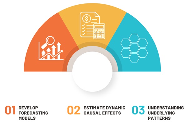
Time series analysis is widely used to:

1. Develop forecasting models: Forecasting future values is one of the primary goals of time series analysis. For example, if a company wants to predict future sales or inflation, time series models can help estimate the future trajectory based on past data.
2. Estimate dynamic causal effects: Time series analysis helps estimate how changes in one variable may affect others over time. For instance, if the Federal Reserve raises interest rates, how will this affect inflation or unemployment rates in the following months?
3. Understanding underlying patterns: Time series analysis helps understand the patterns in the data, which may be essential for decision-making in fields such as economics, business, or environmental management.

What is Time Series Data?

Time series data refers to a set of observations made over time, typically at equally spaced intervals. These observations can represent various types of measurements, such as monthly unemployment rates, daily stock prices, or hourly temperature readings.

Time series data is characterized by the fact that the observations are dependent on time, meaning that each data point is related to previous and future points. This dependency is called autocorrelation, where a value at a given time point is correlated with the value at earlier or later times.

Time series data can be categorized into two types:

1. Discrete time series: Observations are made at fixed intervals (e.g., daily, weekly, yearly).
2. Continuous time series: Observations are made continuously over time.

In practice, time series data is usually discrete, where observations are recorded at fixed, regular intervals. For instance, we may have daily exchange rate data for a year or quarterly GDP data over 20 years.

Features

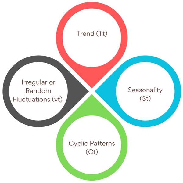
A typical time series can have several components:

1. Trend (Tt): This represents the long-term movement in the data. Trends can be upward, downward, or constant. For example, GDP in many countries tends to show an upward trend over time.
2. Seasonality (St): These are patterns that repeat at regular intervals, often due to seasonal factors. For example, retail sales may spike during the holiday season every year.
3. Cyclic Patterns (Ct): Cycles are long-term fluctuations in the data that are not strictly seasonal. These may correspond to economic cycles, such as recessions or booms.
4. Irregular or Random Fluctuations (νt): These are unpredictable variations that the trend, seasonality, or cyclic components cannot explain. They represent the “noise” in the data.

Types

1. Deterministic Time Series: These series are predictable, with future values determined by a known mathematical function. For instance, a time series based on a known sine wave pattern could be considered deterministic.
2. Non-Deterministic Time Series (Stochastic Time Series): These series have some random component, meaning that future values cannot be predicted exactly but follow a probabilistic distribution. This is the more common case in real-world data, where both known and unknown factors influence the future.

Key Components

Time series data can typically be decomposed into the following components:

1. Trend: The long-term movement in the data, either upwards or downwards.
2. Seasonality: Regular, repeating patterns that occur at fixed intervals (e.g., annual cycles).
3. Residual (or noise): Random fluctuations that are not explained by the trend or seasonal components.

Example

Let’s take the example of inflation rates in the United States. The inflation rate is typically measured by the quarterly percentage change in the Consumer Price Index (CPI) on an annualized basis. If we have inflation data for the past 20 years, we would have 80 observations in total (20 years × 4 quarters per year = 80).

Analyzing this data helps us to identify trends (e.g., rising or falling inflation), seasonal effects (e.g., holiday-related price hikes), and cyclic fluctuations (e.g., economic recessions affecting inflation).

Technical Challenges in Time Series Analysis

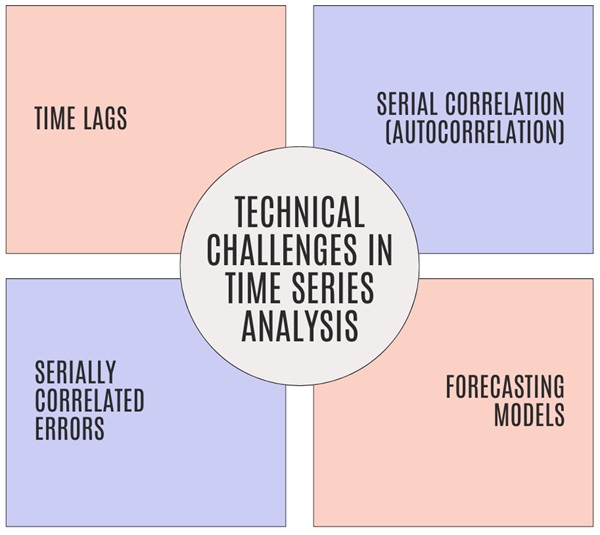
Working with time series data presents several challenges:

1. Time lags: Events in time series data may not affect the series immediately but rather after a delay. For example, changes in interest rates by the Federal Reserve may take several months to influence inflation or unemployment.
2. Serial Correlation (Autocorrelation): This refers to the correlation of a variable with itself over time. In time series data, observations are often not independent, so past values can influence future ones. For example, today’s stock price may be closely related to yesterday’s price.
3. Forecasting Models: Time series forecasting often involves using autoregressive models or other regression methods. Some common methods include:
   • Autoregressive (AR) Models: These models predict future values based on a weighted sum of past values.
   • Autoregressive Distributed Lag (ADL) Models: These are similar to AR models but include both past values of the dependent variable and explanatory variables.

These models are often used for forecasting purposes, even though they may not imply a direct causal relationship between the variables.

4. Serially Correlated Errors: When errors in a model are correlated over time, it complicates the estimation of standard errors and the reliability of the model’s predictions.

Examples of Time Series

Example 1: Australian Red Wine Sales

An example of time series data is the monthly sales of red wine in Australia from January 1980 to October 1991. This data shows how much red wine (in kiloliters) was sold each month, and the analysis reveals trends, seasonality, and potential cyclical patterns in the sales. A notable feature of this data is its seasonal pattern, where sales peak in winter (around July) and dip in the summer months (around January).

Example 2: All-Star Baseball Games Results

Another example is the results of the All-Star baseball games from 1933 to 1995, where the outcome of each game (National League vs. American League) is recorded as either +1 or -1. This data highlights the importance of categorical time series where observations only take specific values (in this case, ±1).

Example 3: Accidental Deaths in the USA

The monthly number of accidental deaths in the USA from 1973 to 1978 is another typical time series. It shows a seasonal pattern, with deaths peaking in the summer months (July) and reaching their lowest point in February. Unlike the wine sales data, however, this series does not show a clear upward or downward trend, making it a good example of seasonal variation without a trend.

Example 4: US Population Growth (1790-1990)

The population of the United States measured every decade from 1790 to 1990 is a clear example of a time series with a long-term increasing trend. This data could be modelled using a quadratic or exponential growth model.

Example 5: Strikes in the USA

The number of labor strikes in the USA from 1951 to 1980 fluctuated significantly over the years. This time series shows no clear trend but fluctuates around a slowly changing level, illustrating irregular cycles and periods of high or low labor strikes due to external factors.

Objectives of Time Series Analysis

The primary objective of time series analysis is to draw meaningful conclusions from the observed data. This can include:

1. Identifying trends: Understanding if the data shows a long-term increase or decrease.
2. Seasonal patterns: Recognizing repeating cycles at regular intervals (e.g., monthly, yearly).
3. Noise and irregular components: Distinguishing between genuine patterns and random fluctuations.

Once the underlying structure is understood, the model developed can be used for various purposes:

• Forecasting: Predicting future values based on past observations.
• Seasonal adjustment: Identifying and removing seasonal effects to analyze other underlying patterns.
• Signal extraction: Filtering out noise to focus on important patterns or trends.
• Model validation: Ensuring that the model accurately represents the data and can be generalized for future predictions.

Stationarity and Its Importance

When working with time series, stationarity is a key assumption. A stationary time series has statistical properties (such as the mean and variance) that do not change over time. This is important because many time series models, like ARIMA (AutoRegressive Integrated Moving Average), assume stationarity.

1. Strict Stationarity: A time series is strictly stationary if its statistical properties (such as distribution) do not change over time. This is a very strong assumption and is often not realistic in practice.
2. Weak Stationarity: A weaker condition, where a time series is stationary if its mean and variance remain constant over time and the covariance between values only depends on the distance between them, not on the actual period.

Also See: Lean Six Sigma Certification Programs, Jersey City, New Jersey

Time Series Forecasting

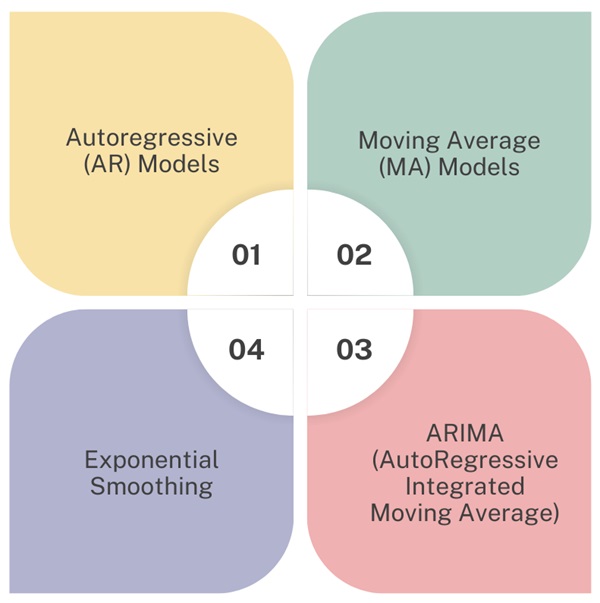
Forecasting future values in a time series involves identifying and modelling the underlying patterns (trend, seasonality, noise) and using this model to predict future observations. Some common models used for time series forecasting include:

1. Autoregressive (AR) Models: These models predict future values based on a linear relationship with past values.
2. Moving Average (MA) Models: These models predict future values as a weighted average of past observations.
3. ARIMA (AutoRegressive Integrated Moving Average): This model combines autoregressive and moving average models and is often used for non-stationary time series after differencing the data to achieve stationarity.
4. Exponential Smoothing: This method uses weighted averages of past observations, with more weight given to more recent observations, making it suitable for time series with trends and seasonality.

Methods for Time Series Forecasting

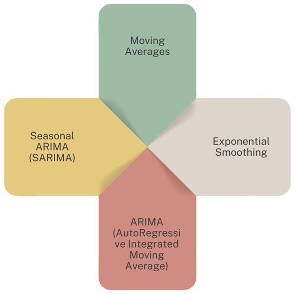
Forecasting is one of the central tasks in time series analysis. Several methods are used for forecasting, including:

1. Moving Averages: A simple method that uses the average of the last few observations to predict the next value. It works well for data without a strong trend or seasonal component.
2. Exponential Smoothing: This method gives more weight to recent observations, making it useful for data with trends and seasonality. It includes variations like simple, double, and triple exponential smoothing, depending on the complexity of the data.
3. ARIMA (AutoRegressive Integrated Moving Average): ARIMA models are widely used for time series forecasting. They combine autoregressive (AR) terms, moving average (MA) terms, and differencing to make the series stationary (i.e., to remove trends and make the variance constant over time). ARIMA models are particularly useful when data shows no clear seasonality.
4. Seasonal ARIMA (SARIMA): This is an extension of ARIMA that accounts for seasonality by including seasonal autoregressive and moving average terms.

Applications of Time Series Models

1. Economic Forecasting: Time series analysis is widely used in economics to forecast key indicators like GDP, unemployment rates, and inflation. By analyzing historical economic data, we can make informed predictions about future economic conditions.
2. Stock Market Analysis: Financial markets are classic examples of time series data. Stock prices, commodity prices, and currency exchange rates are all influenced by trends, cycles, and random events. Predicting future movements in these markets is a key application of time series analysis.
3. Energy Demand Forecasting: Utility companies use time series models to predict future energy demand based on historical consumption data. This helps them optimize power generation and distribution.
4. Weather Forecasting: Meteorologists use time series data from weather stations to predict temperature, precipitation, and other climatic variables.
5. Healthcare Data: Time series analysis is used in healthcare to monitor patient vitals, disease outbreaks, or hospital admissions, providing important insights for planning and resource allocation.

Challenges in Time Series Analysis

1. Non-Stationarity: Many real-world time series are not stationary, meaning their statistical properties change over time. This can make forecasting and modelling more difficult.
2. Seasonality: Identifying and accounting for seasonal variations in the data is essential to avoid misleading conclusions. Seasonality can often mask underlying trends or cause overfitting.
3. Noise: Time series data often contains a lot of random noise, which can obscure the true patterns. Filtering this noise while retaining important signals is a key challenge in time series modelling.
4. Missing Data: Time series data may have gaps or missing observations, especially if the data collection process is not continuous. Proper handling of missing data is crucial for accurate analysis.

Final Words

Time series analysis is a powerful tool for understanding and forecasting data that is collected sequentially over time. It is widely used in various fields, from economics to healthcare, providing valuable insights for decision-making. By identifying patterns such as trends and seasonality, and selecting the right models, time series analysis allows us to predict future events, optimize operations, and make informed decisions.

However, the complexity of real-world time series data—particularly issues like non-stationarity, noise, and missing data—requires careful modelling and validation. With the right approach and techniques, time series analysis can provide deep insights and valuable forecasts that inform a wide range of applications.

Related Articles

• Using the Time Series Plot in Minitab to Show Changes in the Y (or Output)
• Average
• Bullwhip Effect
• Time Plot
• 10 Simple Steps to a Lean Six Sigma Project that Will Get Amazing Results Every Time!