
Have you ever wondered why some assembly lines move faster than others, or why a specific IT system always feels slow? You know there is a problem, and you want a simple way to measure it. The secret often lies in a powerful, yet simple, concept known as Little’s Law. This principle gives you a direct link between the number of items in a system, how fast they enter and leave, and how long they take to move through.
You may feel overwhelmed when you think about managing complex workflows, whether they involve manufacturing parts or processing customer requests. Little’s Law simplifies this challenge. It provides a foundational formula that applies everywhere—from call centers and software development to hospital emergency rooms.
We will not only define this law, but also explore its core formula, understand its assumptions, and show you how to use it to gain vital insights into your own operations. By the end of this article, you will see how this simple but powerful relationship can significantly improve your flow.
Table of contents
Little’s Law Definition
Let us understand the core concept. Little’s Law is a theorem in queueing theory which describes the relationship between three key metrics in a stable system. The law is named after its creator, John D.C. Little. He provided a formal proof for this relationship in 1961.
In simple terms, Little’s Law provides a way to calculate one of three variables if you know the other two. It establishes a necessary and often surprising connection between the number of items waiting and the time each item spends waiting. This means you do not need to know the specific details of the system’s process or how items are served.

Public, Onsite, Virtual, and Online Six Sigma Certification Training!
- We are accredited by the IASSC.
- Live Public Training at 52 Sites.
- Live Virtual Training.
- Onsite Training (at your organization).
- Interactive Online (self-paced) training,
The Little’s Law Formula
The Little’s Law formula is nothing but a straightforward algebraic relationship. It is one of the most vital concepts for anyone studying queueing theory or system performance.
The fundamental formula is:
L = λ × W
Let us understand what these three variables mean:
| Variable | Full Name | Definition Pattern | Unit of Measurement |
| L | Average Number of Items in the System (WIP) | L refers to the average number of items or customers present within the defined boundaries of the system at any given time. | Items, Customers, Tasks (dimensionless count) |
| λ | Average Arrival Rate (Throughput) | λ denotes the average rate at which items enter and exit the system. This rate is also known as throughput in a stable system. | Items per unit of time (e.g., tasks/hour) |
| W | Average Time Spent in the System (Lead Time) | W signifies the average time an item spends inside the system’s boundaries, from arrival to exit. This is also known as lead time. | Unit of time (e.g., minutes, days) |
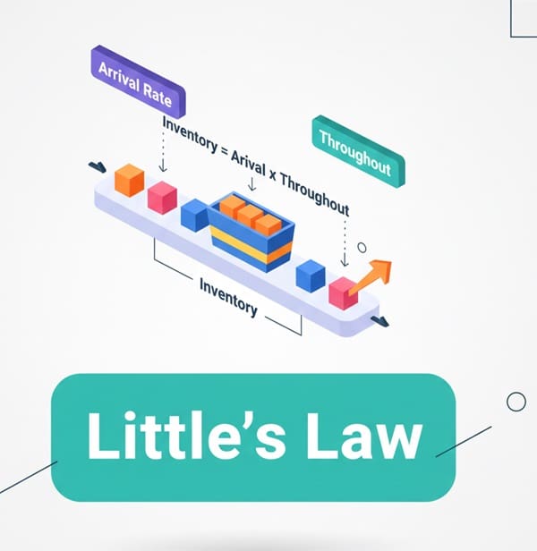
Little’s Law essentially tells you that the average inventory (L) equals the average flow rate (λ) multiplied by the average flow time (W).
Also Read: High-Reliability Organizations: The Blueprint for Flawless Operations
Little’s Law Variables Explained

To understand this better, we must clearly define what each part of the formula represents.
1. Average Number of Items in the System (L)
L means the Work in Process (WIP). It is to be noted that L is a measure of inventory. L is nothing but the total count of all items, tasks, or customers currently active within the system.
For example, if you are managing a software development process, L comprises all features that the team is currently working on or that are waiting to be worked on. In a coffee shop, L includes all customers waiting to order, ordering, or waiting for their drink.
2. Average Arrival Rate (λ)
λ refers to the speed at which new items arrive and enter the system’s boundary. In a stable system, the average arrival rate (λ) must equal the average exit rate, which we call the throughput.
Throughput is a crucial metric as it measures the system’s productivity. It is the number of items that the system successfully completes over a period. Therefore, a faster arrival rate of new work than the exit rate leads to a growing L, which means a buildup of work.
3. Average Time Spent in the System (W)
W is nothing but the lead time or cycle time. This signifies the total duration an item spends within the system, from the moment it enters until the moment it leaves.
W includes both the actual processing time and any time spent waiting in queues. Average time spent in the system provides a direct measure of how efficient your entire process is from a customer’s perspective.
Question: What does a high value for W imply? A high W indicates a slow system, often because the work is spending too much time waiting.
Little’s Law Assumptions: When Does the Formula Work?

Little’s Law is a powerful concept, but it works only under specific conditions. You must understand these assumptions to apply the law correctly and interpret the results accurately.
The core assumptions are:
1. The System is Stable
Stability is a fundamental requirement. Little’s Law depends on the system being stable. This means that, over a long-term average, the average arrival rate (λ) is equal to the average departure rate (throughput).
This implies that the queue is not continuously growing or shrinking indefinitely. If the work is arriving faster than the system can process it, the queue will grow forever, and the law will not hold true for long-term averages. In short, the system must eventually process all the work that enters it.
2. The System is Non-Preemptive and First-In, First-Out (FIFO)
While Little proved the law holds regardless of the specific service time distribution or arrival process, the most straightforward and intuitive application assumes a FIFO system (First-In, First-Out).
FIFO means that the items leave the system in the same order they entered. For most practical purposes, like a line of customers or a sequence of tasks, this assumption helps in interpreting W as the typical time a single item experiences.
3. The Definition of the System Boundary is Clear
Little’s Law requires a clearly defined system boundary. This means that you must clearly identify where an item is considered “in the system” (start of W and L) and where it is considered “out of the system” (end of W and L).
It is critical to be consistent. For example, if you define the system as “from code commit to production release,” you must measure L and W only within those two points.
4. All Items Eventually Leave the System
This means that every item that enters the system must eventually be processed and exit. The system cannot lose items or have them sit in the queue forever. This ensures that the arrival rate and the throughput are equal over the measurement period.
Also Read: Manual Testing Tools and the Software Testing Process
How to Apply Little’s Law?
Little’s Law is not just an academic concept; it is a powerful tool for capacity planning and process improvement in various real-world scenarios.
Using Little’s Law in Service Operations
Consider a customer support call center. We define the system as the time a customer is put on hold until they hang up after the call is resolved.
Scenario: A manager measures that, on average, there are 30 customers waiting for or currently speaking with an agent (L = 30). The center handles an average of 15 calls per hour (λ = 15 calls/hour).
Question: What is the average time a customer spends in the system (W)?
Calculation:
L = λ × W
30 customers = (15 customers/hour) × W
W = 30 / 15 = 2 hours
This means that, on average, a customer spends 2 hours in the call center system, from first contact to resolution. This is a key insight.
Using Little’s Law in Software Development (Agile/Kanban)
In a Kanban system, the primary goal is to limit the Work in Process (WIP) to increase flow and reduce lead time. Little’s Law provides the mathematical backing for this approach.
Here, the system is the entire development process (Ready-to-Deploy).
Goal: The team wants to achieve an average lead time (W) of 4 days for a task. They measure their current average throughput (λ) as 1 task per day.
Question: What is the maximum desirable WIP (L)?
Calculation:
L = λ × W
L = (1 task/day) × (4 days)
L = 4 tasks
This indicates that the team should limit their Work in Process to a maximum of 4 tasks to achieve their 4-day lead time goal. This helps in focusing the team.
Little’s Law vs. Capacity and Utilization
While Little’s Law is a simple formula, we often confuse it with other performance metrics like system capacity and utilization. It is important to understand the key differences.
Comparison Chart: Little’s Law, Capacity, and Utilization
| Basis for Comparison | Little’s Law (L = λ × W) | System Capacity | Utilization (ρ) |
| Concept Denotes | Relationship between Inventory, Flow Rate, and Flow Time. | The maximum possible throughput the system can achieve. | The fraction of time a resource is busy processing work. |
| Formula | L = λ × W | C = 1 / Ts (where Ts is service time) | ρ = λ / C or ρ = λ × Ts |
| Focuses On | Average performance metrics over a period. | The absolute limit of the system’s processing capability. | The busyness or efficiency of the server/resource. |
| Practical Use | Predicting the impact of changing WIP on lead time. | Setting realistic limits for the arrival rate (λ). | Identifying potential bottlenecks and predicting queue growth. |
| Key Insight | The only way to reduce W without changing λ is to reduce L. | Arrival rate must be less than capacity (λ < C) for a stable queue. | High utilization (near 100%) severely increases W. |
The Role of Utilization
Utilization (ρ) refers to the fraction of time a server or resource is actively working. High utilization (e.g., above 80%) leads to significantly longer average time spent in the system (W). This is because any small increase in the arrival rate (λ) forces items to wait much longer for an available resource.
This phenomenon is described by the Pollaczek–Khinchine formula, but Little’s Law ensures that the relationship L = λ × W still holds, even as W increases due to high utilization. We must manage utilization carefully.
Also Read: How can Six Sigma Help Marketers?
Applications of Little’s Law
The core principles of Little’s Law enable us to manage and predict performance in diverse systems.
1. Inventory Management
In manufacturing or logistics, L is the average inventory level, λ is the average demand (sales/consumption rate), and W is the average time inventory sits on the shelf (holding time).
Action: If a business wants to reduce the time inventory is held (W), they must reduce the average inventory (L), assuming the sales rate (λ) remains constant. This helps in freeing up capital.
2. Process Management (Lean and Six Sigma)
Little’s Law is a core concept in Lean methodologies, especially Kanban.
Principle: Limiting the Work in Process (L) is the most effective way to reduce the lead time (W) without forcing people to work faster (changing λ). This is a strategic choice.
3. Computer Systems and Networking
In a computer system, L can be the average number of packets in a router queue, λ is the packet arrival rate, and W is the average delay a packet experiences.
Analysis: Network engineers use L = λ × W to evaluate network performance. If the delay (W) is too high, they know they must either reduce the traffic volume (L) or increase the processing capacity to handle a higher λ. This helps in maintaining service quality.
Key Differences and Common Misconceptions
Little’s Law is simple, but we often misunderstand its scope.
Key Difference: Little’s Law is an Average
Little’s Law only deals with long-run averages. It is important to note that the law cannot predict the instantaneous state of the system or the time a single specific item will take.
For example, if W = 1 hour, it means the average time is one hour. Some items may take 5 minutes, and others may take 5 hours, but the average time spent in the system is still 1 hour.
Misconception: The Law Requires a Specific Distribution
As we know that L = λ × W holds true regardless of the specific probability distribution of arrival times or service times. This means that you do not need to assume that customers arrive smoothly or that service times are constant. The law is robust.
Question: Does the law require that the system has only one server? No. Little’s Law applies to the entire system as a whole, irrespective of the number of servers or the complexity of the internal routing.
Frequently Asked Questions (FAQs) About Little’s Law
What is the primary purpose of Little’s Law?
The primary purpose of Little’s Law is to establish a fundamental relationship between the average inventory (L), the average throughput (λ), and the average time spent in the system (W). This helps in measuring and managing flow in any system where things are arriving, waiting, and being served. It is a powerful diagnostic tool.
Why is Little’s Law important in Lean and Agile methodologies?
Little’s Law is vital in Lean and Agile because it mathematically proves that limiting Work in Process (L) is the direct path to reducing lead time (W). The formula W = L / λ clearly shows that if you keep λ (throughput) constant, reducing L must reduce W. This enables flow optimization.
Does Little’s Law work for unstable systems?
No, Little’s Law does not work for unstable systems over an indefinite time. This is because the law relies on the system being stable, where the average arrival rate (λ) and the average departure rate (throughput) are equal. If the arrival rate is permanently higher than the departure rate, the number of items in the system (L) will grow indefinitely, and the average value will not stabilize.
What is the difference between Lq and L?
L refers to the average number of items in the entire system (waiting plus being served). Lq refers to the average number of items waiting only in the queue (not yet being served). The law L = λ × W is for the entire system, and another related law, Lq = λ × Wq, applies to the queue, where Wq is the average waiting time in the queue.
Key Takeaways
- The formula L = λ × W is universally applicable to any stable system with a clear boundary.
- L is the Work in Process (WIP) or inventory – the average number of items currently in the system at any given time.
- λ is the Throughput or average flow rate – the rate at which items enter and exit the system in a stable state.
- W is the Lead Time or average time spent in the system – the total duration from entry to exit, including waiting and processing time.
- Limiting WIP (L) is the most effective way to reduce Lead Time (W) without compromising Throughput (λ) – this is the mathematical foundation of Lean and Kanban methodologies.
- The law relies on long-term averages and a stable system where work leaves at the rate it arrives – it cannot predict individual item behavior or instantaneous system states.
- Little’s Law is distribution-independent – it works regardless of arrival patterns or service time distributions, making it universally applicable.
- Clear system boundaries are essential – you must consistently define where items enter and exit the system for accurate measurements.
- High utilization dramatically increases lead time – while L = λ × W always holds, W increases exponentially as resource utilization approaches 100%.
- The law applies across diverse domains – from manufacturing and software development to healthcare, call centers, and network engineering, making it one of the most versatile performance management tools.
Final Words
Little’s Law is a cornerstone of queueing theory. This simple but profound formula, L = λ × W, gives you an easy way to connect the three key performance metrics of any stable system: Work in Process (L), Throughput (λ), and Lead Time (W).
Understanding this law allows you to make informed decisions about how to improve your process. If you want a faster system (lower W), you must either reduce the average number of items in the system (L) or increase the processing rate (λ).