Principal Component Analysis (PCA) is a widely used technique in data analysis. It helps simplify complex datasets by reducing their dimensionality while preserving as much of the original information as possible. PCA is part of a broader family of methods. These methods transform high-dimensional data into a lower-dimensional form, making it more manageable and interpretable.
PCA achieves this by identifying the underlying patterns and structures in the data and representing them in new variables, called principal components, which are uncorrelated and easier to analyze.
PCA is used across numerous fields such as machine learning, computer vision, image processing, finance, and psychology. It has become one of the most valuable tools for exploratory data analysis and predictive modelling.
In this article, we will explore the core concepts, mathematical foundation, and practical applications of PCA, along with a step-by-step guide on how it works.
Table of contents
Understanding the Core Concepts
Before delving into the mathematical details, it is crucial to understand some fundamental concepts associated with PCA:
- Dimensionality: Refers to the number of features or variables present in a dataset. For example, a dataset with three variables (height, weight, and age) has a dimensionality of 3.
- Correlation: Measures how strongly two variables are related. A high correlation indicates that when one variable changes, the other also tends to change in the same or opposite direction. Correlation ranges from -1 to +1.
- Orthogonality: In PCA, the principal components are orthogonal, meaning they are uncorrelated with one another. This property ensures that each principal component captures a unique aspect of the data.
- Eigenvectors and Eigenvalues: These are key mathematical concepts in PCA. Eigenvectors represent the directions (or axes) in which the data varies the most, and eigenvalues quantify the amount of variance in those directions. Together, eigenvectors and eigenvalues form the foundation for calculating the principal components.
- Covariance Matrix: This matrix captures the covariance (i.e., the relationship) between pairs of variables in the dataset. A positive covariance indicates that two variables tend to increase or decrease together, while a negative covariance suggests they move in opposite directions.
What is Principal Component Analysis (PCA)?
PCA is a method that helps reduce the dimensionality of data. In simple terms, dimensionality refers to the number of variables or features in a data set. When dealing with large datasets, there are often many variables, which can make it difficult to spot trends or meaningful patterns.
PCA helps by transforming the data into a new set of variables called principal components. These components are ordered by their importance in explaining the variation in the data.. These new components are linear combinations of the original variables, and they capture the most significant patterns in the data.
In addition to simplifying data, PCA also helps in identifying correlations between variables. If certain variables in the data are highly correlated, PCA combines them into one principal component. This reduces redundancy and makes the data easier to analyze.
How Does PCA Work?
PCA works by finding the directions, or axes, in which the data varies the most. These directions are called the principal components. The first principal component represents the direction of greatest variance in the data, and the second principal component is orthogonal (at a right angle) to the first and captures the next greatest variance, and so on.

The general steps involved in PCA are as follows:
- Standardize the Data: If the data includes variables measured on different scales (such as height in meters and weight in kilograms), it’s important to standardize them so that each variable contributes equally to the analysis.
- Calculate the Covariance Matrix: The covariance matrix captures the relationships between the variables. It tells us how the variables are related to each other and how they vary together. The covariance matrix is central to PCA because it helps to identify the directions of maximum variance.
- Compute the Eigenvectors and Eigenvalues: The eigenvectors of the covariance matrix represent the directions (or axes) along which the data varies. The eigenvalues associated with these eigenvectors tell us how much variance each direction (principal component) explains in the data. The higher the eigenvalue, the more important the corresponding eigenvector is in capturing the data’s variance.
- Sort the Eigenvectors: Once we compute the eigenvectors and eigenvalues, we rank the eigenvectors. We rank them based on their eigenvalues in descending order. The first eigenvector corresponds to the direction of greatest variance, the second to the second greatest variance, and so on.
- Select the Top Components: By selecting the top few eigenvectors (those with the largest eigenvalues), we can reduce the dimensionality of the data. These top components capture the most important information in the data, allowing us to work with fewer variables without losing much of the data’s original structure.
- Transform the Data: Finally, we project the original data onto the selected principal components to create a new, lower-dimensional dataset.
Mathematical Foundation of PCA

PCA relies on linear algebra concepts such as matrices, eigenvalues, and eigenvectors. The objective of PCA is to reduce the dimensionality of the dataset while retaining as much variance as possible. The key steps involved in PCA are as follows:
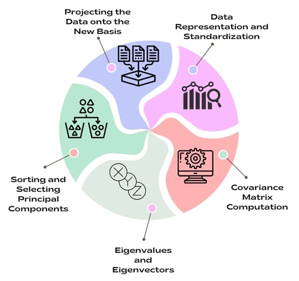
a) Data Representation and Standardization
PCA begins with a dataset represented as a matrix, where each row corresponds to an observation (data point), and each column represents a variable (feature). If the data is not already centred (i.e., each variable should have a mean of 0), the first step is to standardize it. This means subtracting the mean of each variable from the data points.
b) Covariance Matrix Computation
Next, we compute the covariance matrix, which helps us understand how the variables in the dataset are related to each other. The covariance matrix is symmetric, and its diagonal elements represent the variance of each variable, while the off-diagonal elements represent the covariances between pairs of variables.
c) Eigenvalues and Eigenvectors
Once we have the covariance matrix, the next step is to find its eigenvalues and eigenvectors. The eigenvectors represent the directions in which the data has the most variance. These directions are the principal components. The eigenvalues indicate how much variance each eigenvector captures. The eigenvector with the largest eigenvalue corresponds to the first principal component, which captures the most variance in the data. The second eigenvector captures the next largest variance and so on.
d) Sorting and Selecting Principal Components
After calculating the eigenvectors and eigenvalues, we sort them in descending order based on the magnitude of the eigenvalues. This step ensures that the principal components with the highest variance are selected first. We then choose the top k eigenvectors (where k is the desired dimensionality of the reduced dataset) to form a new matrix of principal components.
e) Projecting the Data onto the New Basis
Finally, we project the original data onto the new set of principal components. We do this by multiplying the original data matrix by the matrix of selected eigenvectors. The result is a new set of features (principal components). These features are uncorrelated with each other, and the dataset is now in a lower-dimensional space.
Example
Let’s explore a simple example to understand PCA better. Imagine we have data on food consumption in different countries. We want to analyze the consumption of 17 different types of food in four countries: England, Wales, Scotland, and Northern Ireland.
At first glance, this data is difficult to interpret. Each country has a 17-dimensional data point (one for each food type), and it’s hard to identify any patterns just by looking at the numbers. One way to analyze this data is to plot pairwise relationships between the variables, but for large datasets with many variables, this approach quickly becomes impractical.
PCA comes to the rescue here by reducing the data’s dimensionality. We start by finding the direction of maximum variance in the data, which is the first principal component. This direction tells us which aspect of the data varies the most across the countries. After projecting the data onto this new direction, we can see that the countries cluster into two groups. England, Wales, and Scotland are grouped together, while Northern Ireland stands apart.
Next, PCA identifies the second principal component, which is orthogonal to the first. This allows us to capture additional variance in the data, providing further insights. When we plot the data on these two principal components, we can see even more clearly how the dietary habits of England, Wales, and Scotland differ from those of Northern Ireland.
In this case, PCA has reduced the original 17-dimensional data to just two dimensions, but we’ve still captured 97% of the variation in the data. This reduction in dimensionality makes it much easier to understand and interpret the data.
Also See: Lean Six Sigma Certification Programs, Lincoln, Nebraska
Process

Let’s walk through the steps of PCA algorithmically:
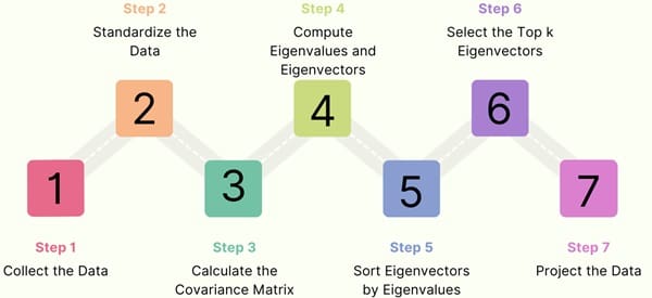
Step 1: Collect the Data
We start by collecting the dataset, which consists of observations and their corresponding features.
Step 2: Standardize the Data
Next, we standardize the data to ensure that all features have zero mean and unit variance. This is important because features with higher variance may disproportionately influence the results of PCA.
Step 3: Calculate the Covariance Matrix
Once the data is standardized, we compute the covariance matrix. This matrix reveals how each pair of features in the data is correlated.
Step 4: Compute Eigenvalues and Eigenvectors
We then calculate the covariance matrix’s eigenvalues and eigenvectors. The eigenvectors define the directions of maximum variance, and the eigenvalues indicate the amount of variance captured by each eigenvector.
Step 5: Sort Eigenvectors by Eigenvalues
We sort the eigenvectors in descending order of their corresponding eigenvalues to prioritise the principal components that capture the most variance.
Step 6: Select the Top k Eigenvectors
We select the top k eigenvectors based on the sorted eigenvalues, where k is the desired number of dimensions in the reduced dataset.
Step 7: Project the Data
Finally, we project the original data onto the new set of selected eigenvectors (principal components). This results in a new, lower-dimensional dataset where each dimension represents a principal component.
Principal Components in PCA

The result of PCA is a set of principal components that are linear combinations of the original features. The number of principal components is equal to or less than the number of original features. The key properties of principal components are:
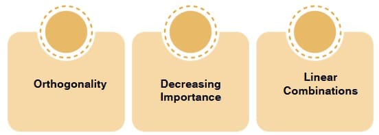
- Orthogonality: Principal components are orthogonal to each other, meaning they are not correlated. This ensures that each component captures a distinct aspect of the data.
- Decreasing Importance: The first principal component (PC1) captures the most variance in the data, while the second principal component (PC2) captures the second most variance, and so on. Thus, the first few principal components usually contain the most important information.
- Linear Combinations: Each principal component is a weighted combination of the original features. These weights are determined by the eigenvectors, and they help describe how each feature contributes to the principal components.
Applications of PCA
PCA is used in various fields for different purposes. Its primary applications include dimensionality reduction, exploratory data analysis, and feature extraction. Some of the notable applications are:
Image Processing
PCA widely compresses images and performs face recognition. It reduces the dimensionality of image data, allowing storage with fewer resources while maintaining key features like shapes and textures.
Data Compression
PCA reduces dataset sizes, making them easier to store and process. This is especially useful in fields like image and video compression, where high-dimensional data must be stored efficiently without losing significant detail.
De-noising Signals
In signal processing, PCA removes noise from signals. It transforms the data into its principal components, isolates the important features of the signal, and discards the noise.
Blind Source Separation
PCA aids in blind source separation techniques, such as separating audio sources from a mixed recording. It analyzes the principal components of the mixed signals and helps separate the individual sources.
Machine Learning
In machine learning, PCA serves as a preprocessing step for various algorithms. It reduces the dimensionality of input data, which improves the performance of models like classification and clustering algorithms.
Data Mining and Psychology
PCA uncovers hidden patterns in large datasets for data mining. It also analyzes complex datasets related to human behavior in psychology.
Bioinformatics
PCA applies to genomics and bioinformatics to analyze high-dimensional data like gene expression data. It reduces the data’s complexity, helping identify important genes or patterns that influence biological processes.
Limitations of PCA
While PCA is a powerful tool, it does have some limitations. For example, it assumes that the data is linear, meaning it may not work well with data that has complex non-linear relationships. Additionally, PCA can be sensitive to outliers, which may distort the results. Finally, PCA may not always be able to provide meaningful insights if the data is noisy or if there are not clear patterns in the data.
Final Words
Principal Component Analysis (PCA) is a powerful statistical tool that simplifies complex datasets by reducing their dimensionality while retaining as much of the variance as possible. It helps in uncovering patterns and structures that would be difficult to identify in high-dimensional data.
Through its mathematical foundation and step-by-step process, PCA transforms correlated variables into uncorrelated principal components, enabling more efficient analysis and interpretation. Whether for data compression, pattern recognition, or feature extraction, PCA remains a cornerstone of modern data science and statistical analysis.

About Six Sigma Development Solutions, Inc.
Six Sigma Development Solutions, Inc. offers onsite, public, and virtual Lean Six Sigma certification training. We are an Accredited Training Organization by the IASSC (International Association of Six Sigma Certification). We offer Lean Six Sigma Green Belt, Black Belt, and Yellow Belt, as well as LEAN certifications.
Book a Call and Let us know how we can help meet your training needs.


